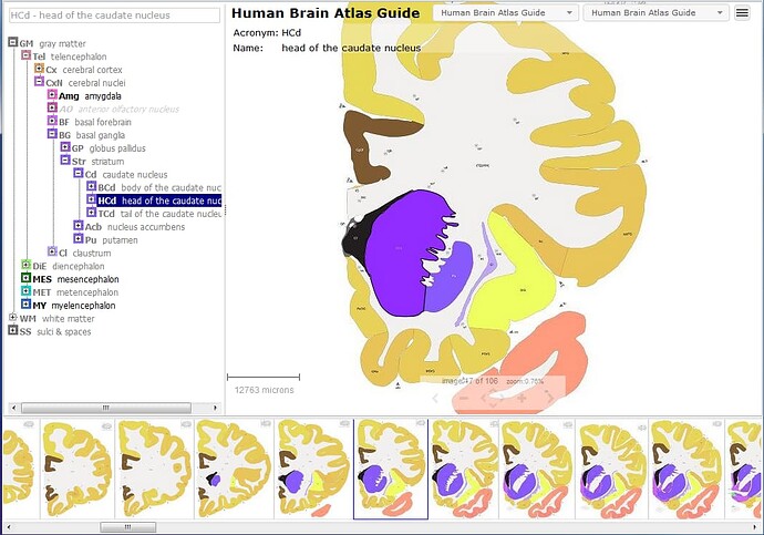
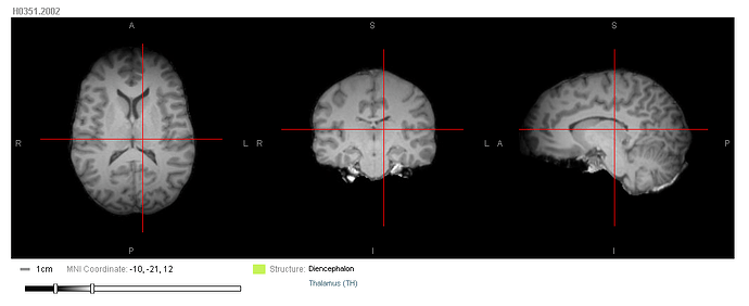
These anatomical reference atlases illustrate the adult human brain, using modified Brodmann or gyral annotation. The Neuroanatomic Reference Guide is meant to provide a spatial context for the anatomic structures of the Adult Human Brain.
The 2D coronal reference atlas is annotated on Nissl sections from a 34-year-old female based on a modified Brodmann nomenclature. It provides spatial context for gene expression in the Allen Human Brain Atlas and the BrainSpan Atlas of the Developing Human Brain. 106 coronal sections at 0.4 - 3.4 mm intervals
The 2D coronal reference atlas is annotated on Nissl sections from a 34-year-old female, by gyrus. It provides spatial context for gene expression in the Allen Human Brain Atlas and the BrainSpan Atlas of the Developing Human Brain. 106 coronal sections at 0.4 - 3.4 mm intervals
Neuroanatomic Reference Guide
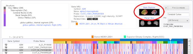
From the heatmap view in the Human Brain Atlas, you can see the Structure Ontology list from the selected data point in the heatmap. Clicking on the link at the bottom of the structure ontology list above the heatmap in the Human Brain Atlas will bring you to the Human Brain Atlas Guide.
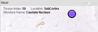
From the In Situ Hybridization data in the Human Brain Atlas, you can also arrive at the Human Brain Atlas Guide by clicking on a hotspot while viewing an experiment in the High Resolution Image Viewer.
Either of these actions will bring you to the Interactive Atlas Viewer with the structure of interest highlighted in purple.
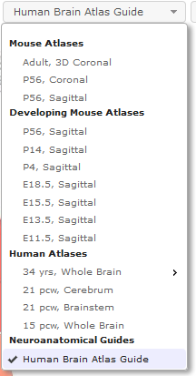
You can also reach this guide by selecting “Human Brain Atlas Guide” from the first drop-down menu in the top right-hand corner whilst in any of the reference atlases in the Interactive Atlas Viewer.
Learn about Human Brain Atlas In Situ Hybridization ISH Data with comprehensive guides and examples from Allen Institute for Brain Science.
Gene expression data is available as colorimetric in situ hybridization (ISH) images for specific brain regions. Images are grouped into image series that comprise an experiment. An experiment consists of a sequence of slides from the same specimen and that receive the same treatment, whether it is Nissl staining or ISH with a probe for a particular gene.
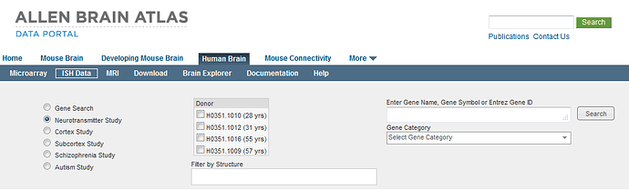
ISH data is available for five distinct studies: The Cortex Study (1,000 Gene Survey in Cortex), Schizophrenia Study, Autism Study, Subcortex Study and Neurotransmitter Study. Please refer to the In situ hybridization white paper in the Allen Human Brain Atlas Documentation tab for details.
Choose among the following options for retrieving the data:
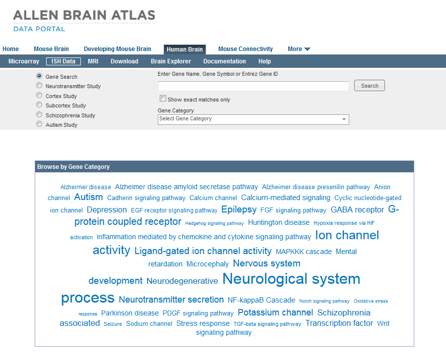
You can search for enhanced gene expression in various categories by selecting on a category from the tag cloud or by selecting multiple categories from the Gene Category drop down menu. The font size in the tag cloud is proportional to the number of genes associated with that category. The categories were created by online search engines such as PANTHER.
Gene Search
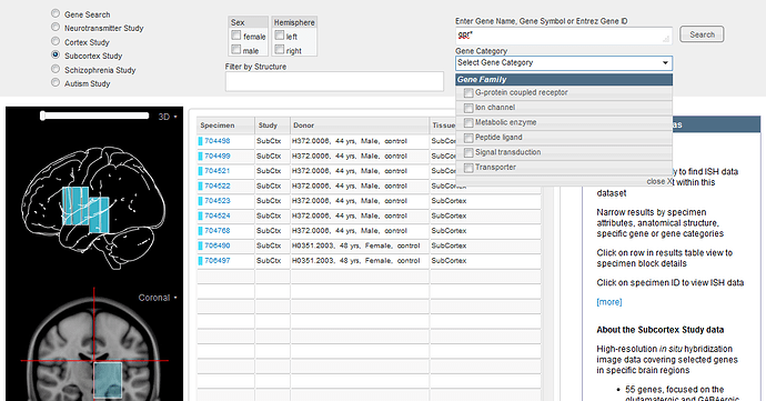
You can search for experiments associated with a gene using its gene symbol, name, or Entrez Gene ID. First, select the “Gene” radio button, type the search term in the input box and click the “Search” button. You will be offered suggestions to choose from while you type, but you can also search by typing the first three or more letters in a gene name or symbol and appending an asterisk ( * ) as a wildcard.
Search by Study
Data includes ISH experiments from five separate projects including: Neurotransmitter Study, 1,000 Gene Survey in Cortex (Cortex Study), Subcortex study, Schizophrenia Study and Autism Study. Please refer to the In situ hybridization white paper and the gene list under the Allen Human Brain Atlas Documentation page for details. A brief description of the study methods are included on the landing page for each study.
You can restrict your search to a single study by selecting the relevant radio button: Neurotransmitter Study, Cortex Study, Subcortex Study, Schizophrenia Study or Autism Study. You will then have a choice to limit your search based on additional criteria such as sex of the donor, hemisphere, etc., depending on the study. Once a radio button for a specific study is selected, you will have the choice to select experiments based on one or more gene categories from the drop-down menu. While in the Subcortex or Neurotransmitter Study (by selecting the appropriate radio button), you also have the option to filter your gene search by structure.
Type a search term in the input box and click the “Search” button. Clicking the “Search” button without an entry in the input box will return the complete list of genes and the accompanying data for that study.
The following search criteria can be specified in the text box to the right of the categories. If you copy and paste in a list of terms delimited by tabs or carriage returns they will automatically be converted into a list of search criteria separated by the OR operator ( | ).
Gene symbol
Gene name
Entrez gene ID
Homologene Group ID
NCBI accession number
Probe name
Boolean Syntax
The following special operators can be used to build queries:
Operator
Example Search Type
Example Query
AND operator: &
Gene
dopamine & receptor
OR operator: l
Gene
ABAT ACHE
NOT operator: !
Gene
“dopamine receptor” !DRD3
AND, OR and NOT may be used in place of their corresponding operators. They must be upper case.
The AND operator (&) is implicit, so spaces between words that are not separated by an operator will be treated like an &.
OR (|) has higher operator precedence than AND (&).
Parenthesis can be used to group criteria, but nested parenthesis are not supported at this time.
The NOT operator (!) is not supported within parenthesis.
Gene Classification
At any time during your visit to this website, you can search on the categories in the tag cloud by selecting the “Gene Classification” radio button and then selecting a category from the drop down menu.
Gene Search Returns
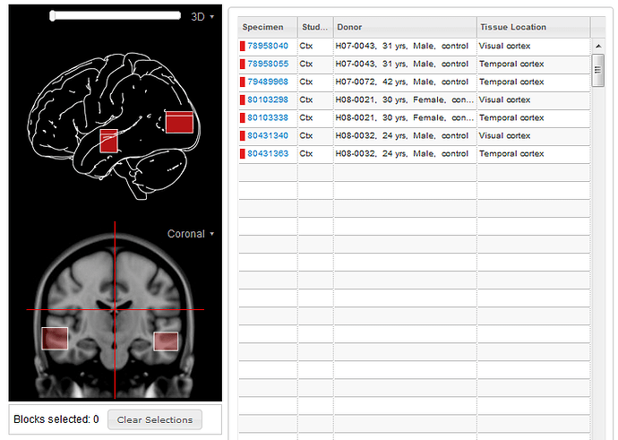
Your search will return a list of specimen blocks which include experiments that fit your search criteria, and an interactive visual display to provide structural context of where the specimen was sampled from. Use the slider bar to rotate the top image, and the drop-down menu to view either coronal or sagittal planes in the lower image. You can filter the search results by clicking on one or more blocks from the visual display. To select more than one block, press Shift and click on the block. Click on the blocks a second time to deselect them or click on the “Clear Selections” button below the display.
The list of experimental returns includes:
Column
Description
Specimen
Clicking on this link will take you to the Specimen Details page
Study
Indicates which ISH Study the sample is from
Donor
Donor Information including: Donor ID, Age, Gender and Disease State
Tissue Location
General location from where the experiment was sampled
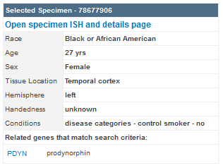
Clicking on the donor will open a panel on the right with more metadata regarding your specimen.
This panel includes demographic information of the donor including their race, gender, age, the tissue location, handedness and any relevant conditions. If your search was not gene specific, all genes that were assayed on this specimen block will be listed under “Related genes that match search criteria:”. You can open the Specimen Detail Information page by clicking the link labeled “Open specimen ISH and details page” or you can directly view the experimental detail by clicking on the gene abbreviation.
Viewing Images
Experiment Details Page
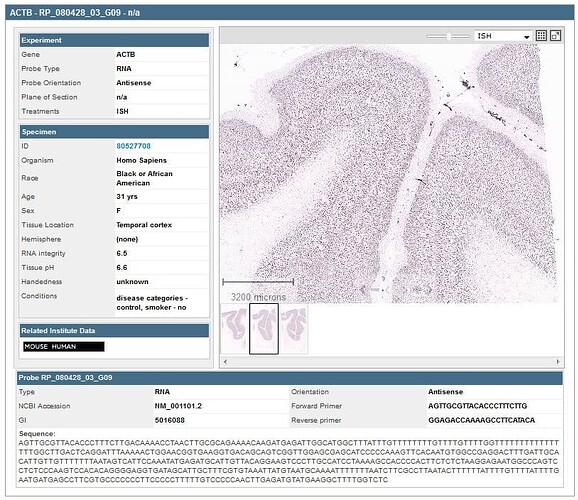
Clicking on the Experiment ID from the search results page will take you to an experimental details page which includes metadata on the experiment, the specimen and the probe as well as related institute data links and a ZAP viewer for all images in the series.
This data can be downloaded as an XML file by clicking the link in “This data is also available as XML”.
Zoom and Pan (ZAP) Image Viewer
The gene symbol or treatment type is displayed in the title bar along with the image series ID. Additional details are displayed across the top of the viewing area, including but not limited to the tissue index and tissue location.
Thumbnails for the entire image series are displayed across the bottom of the viewer in section order. Click a thumbnail to select it for viewing, or use the keyboard to navigate through the set. The current selection is outlined in black.
Scale Bar
Shows the current viewing resolution of the image, in microns. This value dynamically changes as you zoom in/out of the image. You can position the scale bar anywhere on the main image by dragging the scale bar by its ruler.
You can toggle the orientation of the scale bar from horizontal to vertical by clicking on the scale bar text.
Open a new window to view the image series’ details
Close the current image viewer
Keyboard Commands
Key
Description
F
Advance to the next image in the series
D
Go back to the previous image
R
Advance to the last image in the series
E
Go back to the first image in the series
A
Zoom in
Z
Zoom out
Expression Mask Colors
The Expression mask image display highlights those cells that have the highest probability of gene expression using a heat map color scale (from low/blue to high/red).
High Resolution Image Viewer
Side-by-Side Nissl Viewing
Once you click on the full screen viewer button, you will be taken to a screen with side-by-side viewers. The left hand viewer shows the ISH image series and the right hand viewer displays the Nissl image series from the same specimen block. By default, the nearest Nissl section to the ISH image you are interested in will be shown and synched with the section you are viewing. Click the “Sync” checkbox to manually correct any synching between the images. Clicking on another ISH image will automatically display its nearest Nissl section. Clicking on an image thumbnail in the Nissl image series will automatically take you to the nearest ISH image. While the “Sync” box is checked the Pan and Zoom functions will affect both ISH and Nissl images.
Colored circles in the Nissl slides are hotspots - regions that when moused over list the brain regions manually labeled by our Annotation team. Clicking on one of the hotspots will take you to the Interactive Atlas Viewer, which will provide a spatial context for the structure you have indicated inside our Human Brain Atlas Guide.
To download an image, click on the Download icon (see below).
Download Icon
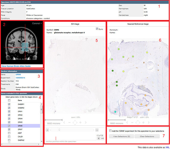
Specimen Detail Information
Clicking on the specimen link from the search results page or on the specimen link in the experiment details page will take you to detailed specimen information. Specimen detail information includes:
Specimen ID - internal ID Age - years Sex - male or female Tissue Location - tissue origination in brain Hemisphere - right or left hemisphere tissue origination RNA Integrity Number - metric indicating RNA integrity from tissue. Ranges from 1 to 10 (degraded to intact RNA) pH - tissue sample pH Race - ethnicity Handedness - right, left, or ambidextrous Conditions - disease conditions, smoker
Spatial Context
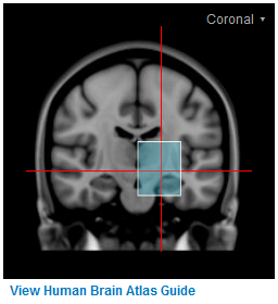
Specimen blocks are drawn onto an MRI image of the donor brain in either the coronal or saggital plane. Click the drop-down menu in the top right-hand corner of the MRI to change orientation.
To view the Human Brain Atlas Guide, click on the link below the image to open an Interactive Atlas Viewer in a new window.
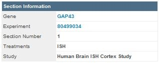
Section Information
The section information box lists information from the current gene pictured in the image viewer including the gene name, the experiment ID, the section number, the treatment and which study the data came from.
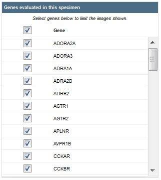
Gene Information
The Gene information section lists the genes that were assayed in this specimen block.
All genes from this specimen block are listed, but only ones selected in your original search criteria are selected. You can select fewer more or less genes/histological stains to view in the image viewer by selecting the checkboxes next to the gene/stain(s) you would like to view.
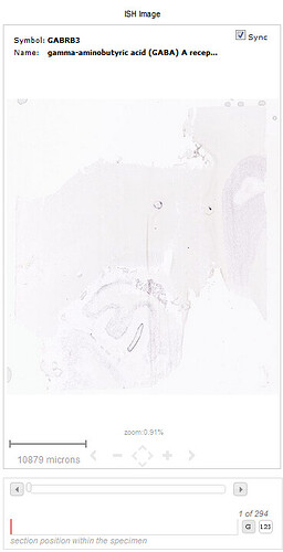
Image Viewer
The viewer displays the image from the current gene highlighted in the gene information box. Below the image is an indicator of the position in the specimen block of that particular section, as well as a visualization of the depth of the section into the block. You can view the sections in order (default or by clicking the 123 button (see below) or grouped by gene button (see below).
123 Button
Gene Button
You can navigate these images similar to the ZAP Image Viewer; with the on-screen navigation tools or the Keyboard Commands.
Nearest Nissl Image
When the “Sync” box is checked in the Image Viewer, the closest reference section will be automatically loaded in this viewer. As you are browsing images in the Image Viewer, the appropriate Nissl image will also be loaded in the reference viewer. The colored spots on the Nissl image are “hotspots” that when hovered over will bring up the structure name and it’s acronym above the image. Clicking on the hotspot will open an Interactive Atlas Viewer with the structure of interest displayed in the context of the brain.
Multiple Experiment Viewer
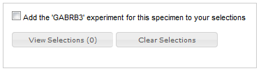
Multiple image series can be opened on the same Web page to enable side-by-side comparisons. If you are interested in seeing separate gene expression experiments in one window together, click the checkbox when you have a gene expression image displayed in the Image Viewer.
You can select as many experiments to view as you’d like and they will be saved until you click the “Clear Selections” button. Once you have selected the experiments you’d like to view, click the “View Selections” button. Once in the Multiple Image Viewer, you can choose a different table layout by clicking on the settings wheel above the viewers and then selecting a different number of columns.
You can swap viewer locations on the page by clicking on one viewer’s title bar and dragging it to another viewer’s location.
Learn about Human Brain Atlas Brain Explorer with comprehensive guides and examples from Allen Institute for Brain Science.
The Brain Explorer 2 software is a desktop application for viewing human neuroanatomy and the Allen Human Brain Atlas microarray gene expression data in 3-D in the framework of the Magnetic Resonance Images of the sampled brains.
System Requirements
Windows Minimum Configuration
Operating System: Microsoft Windows 7 CPU: Intel Core Duo or AMD 1.8GHz System Memory: 1GB Graphics Card: Hardware 3D OpenGL accelerated AGP or PCI Express with 64MB RAM Screen: 1024x768, 32-bit true color Hard Disk: 200MB free space
Note: Brain Explorer is known to work with the following video chipsets: nVidia GeForce 9400/9600, nVidia Quadro FX 1800/3800/5600, AMD Radeon 9600, AMD Radeon HD 3200/4550, Intel Q35/Q45 Express
Important Please install the latest drivers for your video card for best compatibility and performance.
Mac Minimum Configuration
Operating System: OS X 10.6.8 CPU: Intel 1.8GHz System Memory: 1GB Graphics Card: 3D-capable with 64MB RAM Screen: 1024x768, 32-bit millions of colors Hard Disk: 200MB free space
Important Please install the latest system updates from Apple to ensure you have the latest video card drivers.
Installation
Windows
For the best performance, please check with your video card vendor for the latest available drivers before using Brain Explorer. The Windows version of Brain Explorer is available here. Double-click the downloaded BrainExplorer2.msi file and follow the prompts.
Mac
The Mac version of Brain Explorer is available here. Double-click the downloaded zip file to unpack Brain Explorer.
Installing Atlases
A one-time download containing anatomy files is needed following installation of the Brain Explorer application. The first time you open Brain Explorer, you will be asked to choose to download files for the Mouse Brain, Developing Mouse Brain and Human Brain atlases. Click on the atlases you would like to use and then click the Install button.
To download missing atlases on the PC, go to the Help menu and select Download Atlases. On the Mac, the command is in the Brain Explorer 2 menu.
Getting Updates
Brain Explorer will inform you when updates to the Brain Explorer application itself or its atlases are available. New data may not be available for viewing until you install the required updates.
Viewing Gene Expression
To load gene expression data into Brain Explorer: go to the Allen Human Brain Atlas and perform a gene search. You can click on a gene category in the tag cloud or type in a gene in the search box. Your search returns a heat map showing gene expression profiles over different structures in the brain. Click on a cell in the heat map - this selects a sample in your probe of interest. To see the gene expression for the probe you selected in 3D click on the Brain Explorer link to be taken to the Brain Explorer with the sample automatically highlighted.
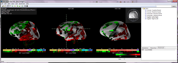
The Image Viewer will automatically show the 3-D expression representations of your gene of interest on every sampled brain. Cortical gene expression is overlaid on an inflated white matter surface for each donor brain, with spots under the cortical surface representing gene expression in the subcortical regions of the brain. Under each representative brain is the heat map for the probe you selected. Clicking on that heat map will pinpoint the area in the brain from which the sample was taken.
The gene expression colors correspond to the settings in the Atlas with which you were viewing the original heat map. To change the gene expression representation, click on the “Gene” tab in the top left hand corner of your screen and choose either Z-score or raw colors.
A compass in the right hand corner of the image viewer depicted by a stylized head can be used to rotate the brains by clicking and dragging your cursor. You can look at a single brain by clicking on the magnifying glass above that brain. The magnifying glass will appear as you hover over the donor ID for each brain. You can also remove a brain by clicking on the “x” next to the magnifying glass.
To restore all views, choose Show All Views from the View menu. Choosing a data point, either by clicking on the heat map below the brain or on a brain region itself, will bring up the gene symbol, the location of the sample and the expression level and z-score in the top left hand corner of the Image Viewer.
You can zoom using either the wheel on your mouse or using the Zoom scroll bar in the lower right hand corner of the Image Viewer.
Structure Ontology Viewer
The Structure Ontology Viewer shows the entire collapsible ontology for the human brain including the color coding used by our expert annotation team to visualize structural boundaries. Two columns to the right of the ontology determine the type of data displayed in the Image Viewer. “A” represents annotation and when checked, will show a visual representation of that structure in the Image Viewer. “G” represents gene expression and when checked, will show gene expression in that structural domain.
The default organization for the Structure Ontology is the Hierarchical View, but if you are unfamiliar with the ontology, you can click on the Alphabetical View to see the structure list in alphabetical order.
The Bookmarks tab is a space where you can create and save favorite views of the brain. Several default views are already saved that will rotate the brain back into common viewing frames.
Gene List
This section displays the gene probes you have selected and downloaded in this session. When more than one gene probe has been downloaded, clicking on one probe will show its gene expression profile in the image viewer. Right clicking on the gene probe name will bring up a menu where you can view the gene detail page (Get Info), be taken to the Planar View of the probe (View Images) or copy the gene information for use in another application.
Using the Toolbar
Button
Operation
Selects cursor rotation tool mode
Selects cursor pan tool mode
Selects cursor selection tool mode
Toggle Sagittal Atlas section viewing
Toggle Coronal Atlas section viewing
Toggle Horizontal Atlas section viewing
Centers the Viewer on the current pinpointed expression data point
Turns on the clipping planes
Toggles the Structure Ontology and Gene List View
Advanced Features
Atlas Tab:
You can show opaque three dimensional structures of the brain by “showing” or “hiding” structures from this menu. The “Transparent” function allows you to see transparent views of the structures to view the anatomical relationships between them.
Selecting the sagittal, coronal or horizontal sections (or clicking on one of the section image buttons in the toolbar) will superimpose a single plane of the MRI images from each brain on your image space. These planes can be moved once the selection tool mode button in the toolbar is selected. Selecting “Show Annotation on Section” from this menu will color the MRI images according to the brain structure ontology.
Gene Tab:
When you have a gene selected, the Gene Tab menu allows to you to show all expression, hide all expression (for instance to then select a single structure) or toggle expression (for instance, unselect your region of interest then toggle to see expression in only that region).
You can also show or remove threshold controls and choose the visual representation of your data (raw data vs. z-score) from this menu.
To be taken to the gene detail page, select “Get Info”. To see the Planar View, choose “View Images”. These functions are also available by right-clicking on the gene name in the Gene List.
Clipping Planes:
When this function is selected, either by toggling the cutting tools button in the toolbar or selecting “Clipping Planes” from the View drop down menu, you can make coronal, sagittal or horizontal cuts in your view of the brain and related data. To cut in a particular plane, make sure the cursor is in selection tool mode, and then click and drag on the plane you are interested in clipping.
Troubleshooting
Windows
Graphics
If you are using a desktop computer, you should obtain drivers from the video card manufacturer. First, identify the video card. Go the Start menu and open the Control Panel. Open the Display control panel and go to the Settings tab. Click the Advanced button and go to the Adapter tab. Your video card vendor and model name will be displayed at the top of the window under Adapter Type. Please go to the manufacturer’s web site, locate the driver download, and follow the instructions on the website or included with the downloaded file.
If you are using a laptop computer, you will need to go to your laptop manufacturer’s web site to locate the latest video drivers.
You can also activate an alternate drawing mode in Brain Explorer. Go to the View menu and select Options. Check the Draw faster but at lower quality button and uncheck the Synchronize drawing with the monitor’s vertical refresh button. Set the Multisample setting to Off.
If you are using multiple video cards from different vendors, the 3D display may not work correctly on all attached monitors.
Uninstalling
Use the Add/Remove Programs control panel or the uninstall link in the Brain Explorer folder in the Start menu. Additional data that are not automatically uninstalled are located at the following locations:
Windows XP
Atlas data: C:\Documents and Settings\userid\Local Settings\Application Data\Allen Institute\Brain Explorer 2 User settings: C:\Documents and Settings\userid\Application Data\Allen Institute\Brain Explorer 2
Windows Vista and Windows 7
Atlas data: C:\Users\userid\AppData\Local\Allen Institute\Brain Explorer 2 User settings: C:\Users\userid\AppData\Roaming\Allen Institute\Brain Explorer 2
Proxy Settings
If you use a proxy server, Brain Explorer will use the proxy settings from the Internet Options control panel in the Windows Start menu. Please refer to the Windows documentation for help on proxy settings.
Mac
Uninstalling
Drag the Brain Explorer 2 icon to the trash. Brain Explorer generates the following files, which can also be dragged to the trash.
If Brain Explorer is not running smoothly, first try to free up as much memory as possible by quitting all other open applications. You can also activate an alternate drawing mode. Go to the Brain Explorer 2 menu and select Preferences. Check the Draw faster but at lower quality button and uncheck the Synchronize drawing with the monitor’s vertical refresh button. Set Multisampling to Off.
Contact Us
If after reading this help file you still have questions or suggestions, please Contact Us.
Learn about Human Brain Atlas API with comprehensive guides and examples from Allen Institute for Brain Science.
The Allen Human Brain Atlas is a multimodal atlas of the human brain that integrates anatomic and microarray-based gene expression information. Microarray sampling sites (~400-1000 sites per brain) were identified by expert anatomists using cytoarchitectural information from multiple histological stains. Sampling site delineations in the high resolution histological images were subsequently mapped into each individual’s MR image space to provide 3-D anatomical context. All brains were also registered to MNI space to enable cross-individual comparisons.
From the API, you can:
Download expression values
Query the correlative and differential search services
Download MRI images
Experimental Overview and Metadata
RNA isolated from each sample area was hybridized to a custom Agilent 8x60k microarray chip to measure gene expression over the transcriptome. All least two different probes were available for 93% of genes. Probes were located on different exons as much as possible when multiple probes were available for a gene. For 60 genes, sets of tiling probes were designed.
Each sampling site was associated to a Structure by expert anatomists using cytoarchitectural information from multiple histological stains. Structures are organized hierarchically into a tree in which children structures are “parts of” their parent structure. Structures are assigned colors that visually emphasize the hierarchical relationships.
Gene expression data for samples passing quality control are normalized to enable cross-comparison between batches of samples processed at different times or samples belonging to different donors. For more details on microarray data generation and processing see the Microarray whitepapers.
Normalized microarray expression values can be downloaded in several ways:
From the web application Download page. Each zip file contains the normalized values for all probes and all samples for one donor )
From the “Download this data” link below the heatmap in the web application.
From the connected data service in the API
All experimental data from this study is associated with the “Human Brain Microarray” Product. All probe and sampling site information can be accessed through the API using RMA queries.
RNA-Sequencing (RNA-Seq) data were generated for a selected set of 240 samples (120 from each brain) representing matched cortical and sub-cortical regions across two brains (H0351.2001 and H0351.2002). The gene expression data (both raw and TPM counts) can be downloaded from the web application Download page.
Through a quantitative comparison of microarray and RNA-Seq data, a set of quality control metrics has been computed for each Agilent microarray probe which allows a user to filter out problematic probes or choose the most reliable probe for each gene. The probe metric table and metadata can be downloaded here.
Downloading Expression Values
Normalized expression values can be obtained by specifying:
a list of probes
a list of donors (optional), and
a list of structures (optional)
See the connected service page for definitions of service::human_microarray_expression parameters.
Example:
Download expression values for donor “H0351.1015” in structure “locus ceruleus” for all probes associated with gene SLC6A.
the Gene (id, acronym, name, entrez-id), along with
a vector of normalized expression values in the same order as the “samples” array.
a vector of z-score values in the same order as the “samples” array. Note: z-score is computed independently for each probe over all donors and samples.
Each sample contains information about:
the Donor (id, name, age),
the Sample (well id and (x,y,z) coordinate in the MR volume in millimeters),
the associated Structure (id, name, acronym and color), and
the associated top (coarse) level Structure (id, name, acronym and color).
Differential Search
The differential search function finds probes that show the greatest difference between two sets (target and contrast) of user-defined structures. For each probe, a 2-sample t-test is performed followed by Benjamini and Hochberg false discovery rate correction. The null hypothesis is that the average expression level of samples in the contrast set of structures is greater than or equal to the average expression level of samples in the target set of structures. A statistically significant result (p-value less than user-defined threshold) allows us to reject the null hypothesis and conclude that the average expression level of samples in the target set of structures is greater than the average expression level of samples in the contrast set of structures. Resulting p-values are sorted in ascending order. Search results can also be sorted by fold-change (log ratio of expression) in descending order.
The differential search function can be accessed through the Web application or using the API.
See the connected service page for definitions of service::human_microarray_differential parameters.
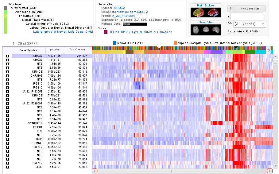
Example: Differential search for genes with higher expression in thalamus than the cerebral cortex
Figure: Screenshot of top returns of a differential search for genes with higher expression in the thalamus than in the cerebral cortex. The z-score heatmap shows enrichment (red) in the thalamus (structure color: light green) relative to other brain regions.
Usage of this service is demonstrated in the SPM example application.
Correlative Search
The correlative search function finds probes with expression profile similar to that of a selected seed probe over all samples within a user-specified structure. Pearson’s correlation coefficient is computed for all probes and the results ranked in descending order.
This correlative search function can be access through the Web application or using the API.
See the connected service page for definitions of service::human_microarray_correlation parameters.
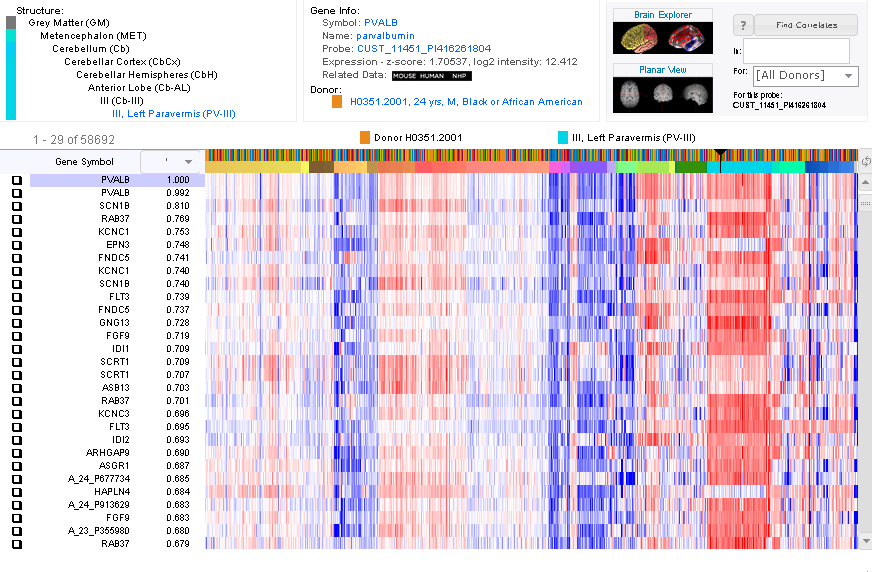
Example: Correlative search for probes with similar expression to PVALB probe CUST_11451_PI416261804 over the whole Brain
Find Probe ID for probe “CUST_11451_PI416261804” (id = 1052410)
Figure: Screenshot of top returns of a correlative search for probes with similar expression to a PVALB probe with expression values displayed as a z-score heatmap.
Magnetic Resonance Imaging
T1-weighted MPRAGE scans were acquired for the postmortem brains using 3T Siemens Trio MR scanners (TI=900ms, TR=1900ms, TE=3.03ms, 9 degree flip angle, 1mm isotropic voxels). Scans were performed in cranio for some brains and ex cranio for others. See the Microarray whitepapers for more specific scan sequence details for each brain.
The T1, T2 and DTI (if available) volumetric data can be downloaded from the Web application or via the API.
All T1 images were registered to MNI space. FreeSurfer’s affine registration was used for the in cranio scans. For ex cranio brains, the T1 was first rigidly aligned using FSL (Jenkinson, et. al, 2002) and then non-rigidly aligned using ANTS (Avants, et. al., 2011). The 3-D affine transform from a location in the MR volume to MNI space is encapsulated in the Alignment3d model.