This third section "Putting it all together" is a key to link research focus to related scientific tool to primary paper to taxonomy used.
Putting it all together
The associated tool::paper::taxonomy::research focus
This table links the research topic (species, brain area of interest, and technique) to the related tool, the related dataset, the related paper, and the related taxonomy.
Related Resources:
Discover all pages in this series:
- Cell Type Support: Introductory resources
- Cell Type Support: Technical Resources
- Cell Type Support: Mapping tools to papers and taxonomies
This second section "How to..." lists more technical resources such as tutorials, protocols, use cases, and more.
How to...?
Technical Protocols, Guides, Useful Supplemental Information
These are Allen Institute resources to explain how to use our datasets, replicate our experiments with protocols, and links to tables with important metadata and features definitions. These sections are designed for scientists who are interested in more technical support in their cell types research.
How to understand cell type nomenclature
Identifying and naming brain cells has been an integral part of neuroscience for a century, including Allen Institute cell typing efforts. This means many cell types have multiple names, and tracking this information requires standards.
1. Understand the Allen Institute framework for developing nomenclatures called the Common Cell Type Nomenclature, or CCN.
Related publication (Miller et al 2020)
2. Learn about the schema the Allen Institute has developed for defining cell type taxonomy components, such as nomenclature, annotations, metadata, and the underlying transcriptomic data, or use this format for your own data.
Allen Institute Taxonomies in AIT Format
3. Compare how cell type names have changed as the Allen Institute collects more data from across the brain, and see how brain region, age, gene counts, and other cell features relate to cell types.
Annotation Comparison Explorer
How to replicate our Patch-Seq protocols and analysis
Adopting the Patch-seq technique in a lab can be daunting, but these protocols and resources can help. The Allen Institute has adopted and extended multiple experimental and computational protocols to make Patch-Seq is a useful method for understand the structure and function of brain defined cell types.
These resources below are used in multiple tools and data sets on Allen Brain Map:
Related tool: Allen Cell Types database
Related tool: Mouse PatchSeq VISp viewer
Related tool: Cell Type Knowledge Explorer
1. This GitHub provides a starting point for labs interested in using the Patch-seq technique or refining their existing technique. Specifically, this resource consists of three components: (1) a step-by-step optimized Patch-seq protocol (2) the Multichannel Igor Electrophysiology Suite (MIES) software package and (3) an R library that uses a modified workflow.
Related publication (Lee et al 2021)
2. Overview of the various steps and tools to generate data across species and brain regions in Patch-Seq.
3. From our electrophysiology team, this is detailed protocol to obtain electrophysiological recordings and cellular contents from neurons in postnatal mouse and/or human brain slices.
Related publication (Lee et al 2021)
4. IPFX is a Python package for computing intrinsic cell features from electrophysiology data. That can perform cell data quality control (e.g. resting potential stability), detect action potentials and their features (e.g. threshold time and voltage), calculate features of spike trains (e.g., adaptation index), and calculate stimulus-specific cell features.
Automatic computing for electrophysiological cell features
5. Here is your one-stop shop for the Allen Institute’s free, open-source neuron reconstruction software, protocols, and analysis scripts for generating and analyzing image-based, quantitative, 3D morphologies for your own research.
Protocol, Software, Analysis: Reconstruct neuron morphology
6. Protocol to generate full-length cDNA from single cells, or nuclei, using Takara SMARTer V4.
Takara SMARTer V4 (Protocols.io protocol)
7. The electrophysiology and morphology feature definitions are used for all our Patch-Seq datasets. This is from “NIHMS1691616-supplement-Supplementary_Figures” in Gouwens, Sorensen, Berg, et al. 2019, starts at page 73 for electrophysiology and page 75 for morphology.
Electrophsyiology & Morphology Features Definition
Related publication (Gouwens et al 2019)
How to replicate our RNA-Seq laboratory protocols
We define cell types based on which genes are turned on and which genes are turned off in a cell. These resources detail how we do this robustly for millions of cells.
1. This page includes protocols for SMART-Seq and Nextera XT, FACs, and tissue preparation and analysis & clustering links.
SOPs: RNA-Seq mouse whole cortex & hippocampus
SOPs: RNA-seq human multiple cortex areas
2. To monitor for a consistent, high-quality sampling of single-cell and single-nucleus RNA-Seq data, we have controls used in each application sample. These controls for mouse and human data are available to download for you to use in your own experiments.
How to use the Cell Type Knowledge Explorer
The Cell Type Knowledge Explorer is a scientific and educational tool for exploration of human, marmoset, and mouse primary motor cortex cell types and the features that make them distinct.
Explore the Cell Type Knowledge Explorer
1. Learn from the scientists behind our Cell Types Knowledge Explorer about why it is made, key findings, and a walkthrough of the tool itself.
2. Read the science behind the cell type knowledge included in the Cell Type Knowledge Explorer in peer-reviewed publications.
Mouse Patch-seq (Scala et al 2021)
Mouse transcriptomics and epigenetics (Yao et al 2021)
Aligning cell types across species (Bakken et al 2021)
3. These use cases were designed to show researchers how to use the mouse data in the Cell Type Knowledge Explorer for their own research questions. The case titled “Experimental Design” shows how the Cell Type Knowledge Explorer can be used to guide research questions.
4. Python code for you to your own generate data visualizations that was used in the Cell Type Knowledge Explorer.
Replicate our data visualization
How to use the Allen Brain Cell (ABC) Atlas
The Allen Brain Cell (ABC) Atlas provides a platform for visualizing multimodal single cell data across the mammalian brain and aims to empower researchers to explore and analyze multiple whole-brain datasets simultaneously.
1. From our product managers of ABC Atlas, here is a user guide to help you navigate all the features of ABC Atlas.
2. The ABC Atlas is under active development! See all the updates & patches to ABC Atlas on the Allen Brain Map Community Forum post that is updated regularly.
ABC Atlas channel on the Community Forum
3. Read the science behind some of the data sets included in the ABC Atlas in peer-reviewed publications.
Mouse Whole Brain (Yao et al 2023)
Mouse Whole Brain (Zhang et al 2023)
Human Whole Brain (Siletti et al 2023)
Human Alzheimer's disease (Gabitto et al 2021)
4. These use cases were designed to show researchers how to use the Whole Human Brain data in the ABC Atlas for their own research questions. The two use cases titled “Experimental Design” show how the ABC Atlas can be used to guide research questions, while the use case titled “Scientific Knowledge” shows how the ABC Atlas can be used studying and/or writing a literature review. The “coding” in the third use case shows users how to access the raw data for the Whole Human Brain using Jupyter notebooks.
Use Case: Scientific Knowledge
Use Case: Experimental Design with Coding
5. Learn from the scientists behind the new collection of studies from the BRAIN Initiative Cell Atlas Network (biccn.org) and published in Nature on Dec 14, 2023.
Whole Mouse Brain Paper Package Highlights Webinar
Related Collection of Scientific Publications
6. List of the 500 Gene panel used in the whole brain mouse. This is from the supplemental table 6 in Yao, et al. 2023. Also, the set of genes where expression in the spatial transcriptomics data is estimated (or "imputed") using information from the single cell RNA-seq data.
Whole Mouse Brain, Spatial Gene Panel List
Whole Mouse Brain, Spatial Imputed Genes
7. Tables including detailed information for each cluster, including neurotransmitter information, overall marker genes, main dissection region, and more. The first two buttons correspond to clusters in whole mouse brain (supplemental table 7 in Yao et al 2023) as published, and updated to include a comparison with clusters in a previous study of mouse cortex and hippocampus (Yao et al 2023). The third button relates to subclusters in whole human brain (unpublished supplemental information from Siletti et al 2023).
Whole Mouse Brain, Published Cluster Annotation Table
Whole Mouse Brain, Extended Cluster Annotation Table
Whole Human Brain, Subcluster Annotation Table
8. Download Excel files of the acronyms found in ABC Atlas with their corresponding full name, type of acronym (“types”), and the identifiers (“primary identifier”, “secondary identifier”, and “tertiary identifier”). See the table below for list of the types and identifiers used in the Excel file. Note that acronyms are now defined directly in the ABC Atlas in 'nomenclature cards'.
Whole Mouse Brain Cluster Annotations
Whole Mouse Brain Anatomical Annotations
Whole Human Brain Cluster Annotations
ABC Atlas Dataset Descriptions
An ever-growing number of data sets are included in the ABC Atlas. This table lists the names, relevant publication, names and number of data points for every data sets available on the ABC Atlas (as of September 2025).
How to use the MapMyCells
MapMyCells allows you discover what cell types your transcriptomics and spatial data corresponds with by comparing your data to our massive, high-quality reference datasets.
1. Learn from one of our scientists behind MapMyCells on how to use it, what type of data it accepts, what taxonomies are built of fit, which algorithms to select, and peek under the hood on how it works.
2. MapMyCells needs cell by gene matrix where rows are “cells” and columns are “genes”, which need to be in either a csv, csv.gz, or h5ad file format. This guide provides more details about how to prepare your file, including input file limits.
Input creation, file requirements, and limits
3. Unsure what algorithm or taxonomy to select in MapMyCells? These guides are for you.
4. The online version of MapMyCells will provide accurate cell type assignments for user-inputted data in most cases. However, there are some situations when using the direct scripts may be more appropriate: (1) if the reference taxonomy you are interested in is not one currently included in MapMyCells, (2) if the data set you have is quite large, (3) if you'd like to include these algorithms as part of an analysis pipeline, or (4) if you need to select a different set of genes for mapping (e.g., for mapping MERFISH data).
Run MapMyCells in python (cell_type_mapper)
Run MapMyCells in R (scrattch.mapping)
BICCCN and BICAN
Most of these resources are part of the Brain Initiative Cell Census Network (BICCN) and/or Brain Initiative Cell Atlas Network (BICAN). The Allen Institute serves as the coordinating member of this network.
Related Resources:
Discover all pages in this series:
- Cell Type Support: Introductory resources
- Cell Type Support: Technical Resources
- Cell Type Support: Mapping tools to papers and taxonomies
This first section "What is..." lists introductory information on cell type topics.
What is...?
Introductory resources
Here are Allen Institute resources to help you understand the fundamentals of cell types and the research methods used to study cell types; including Patch-Seq, taxonomies, UMAPs, and more. These sections are designed for those who are unfamilar with cell type topics to help introduce them to the concepts.
What is a cell type?
Cells within a type exhibit similar structure and function that are distinct from cells in other types.
1. Learn from our Executive Vice President & Director of Brain Science, Hongkui Zeng, on the overview of cell types from the roots in evolution & development to the approaches in how to characterize, while also providing a roadmap for the future.
2. Cell Types 101 Webinar focuses on an introduction to the study of cell types! It covers evolving cell type definitions, cell types across species, the types of data used to define cell types, and the importance of having standard definitions for cell types.
What is transcriptomics?
The study of RNA expression (the transcriptome) and how it differs between cells / tissues / conditions.
This webinar is tutorial on Allen Cell Types Database. Starting at 4:13, we give an overview of single cell or nucleus transcriptomics. (Note: Webinar is from 2021; the taxonomies presented in the webinar are not the latest taxonomies from the Institute, as newer taxonomies have been created since 2021.)
This guide book describes how 10x single cell sequencing works with easy-to-understand language and graphics.
What is a (cell type) taxonomy?
A cell type taxonomy is a specific analysis organizing cells into groups (or types), applied to a specific set of data, and saved in a standard format. Cell types are annotated with data-driven and historical information about their characteristics.
1. This user-friendly tutorial goes step by step on how cell type taxonomies are created, with linking to data from Allen Cell Types Database in the end. This is a great web-interface that is perfect for students to experts to begin exploring what a taxonomy is.
Explore the Interactive Walkthrough
Related tool: Allen Cell Types Database
Related Publication (Tasic et al 2016)
2. 'What is a taxonomy?' webinar is focused on the systematic classification of cell types and their hierarchical relationships. Much like species taxonomy (family, genus, species, etc.), researchers at the Allen Institute and their collaborators are working to create a standard taxonomy for cell types.
What is a UMAP?
Uniform Manifold Approximation and Projections (or 'UMAPs') are helpful ways of displaying many types of data and are often referred to as one type of dimensionality reduction tool.
A UMAP is a common way to visualize cell types taxonomies. Learn how to interpret and analyze these graphs in this user guide.
What is Patch-Seq?
Patch-Seq is modified version of Patch-Clamp, with the additional steps of extracting the nucleus to obtain transcriptomics and preserving the cell body to obtain morphology.
1. Patch-Seq was developed around late 2010s, with Allen Institute helping to optimize the technique. Here is a 2016 Allen Institute team talk giving an overview of Patch-Seq.
Watch the Team Talk
See other Patch-seq resources and publications
2. This webinar from 2024 gives an overview of what Patch-Seq is and how that data is used in the Cell Type Knowledge Explorer tool.
Watch the webinar
Explore motor cortex cell types in the Cell Type Knowledge Explorer
Related Resources:
Discover all pages in this series:

Find answers to frequently asked questions about the Genetic Tools Atlas. Learn about viral vectors, transgenic mouse lines, and tool selection.
These frequently asked questions (FAQs) center around the Genetic Tools Atlas, a searchable web tool representing information and data on enhancer-adeno-associated viruses (enhancer AAVs) and mouse transgenes characterized at the Allen Institute for Brain Science.
Learn more about the Genetic Tools Atlas.
Why does it seem like some datasets are repeated across multiple rows?
You are correct that this is the case, and we understand it is not intuitive. For each experiment (same Donor ID), each distinct population of labeled cells is independently scored for its anatomical location (Coarse Labeled- and Fine Labeled ROIs) as well as its labeling brightness and density. In the table format, each row represents an individual score within an experiment, rather than an individual experiment. This format often results in multiple rows belonging to the same experiment. In the planned 2026 release, this layout will be replaced by a more user-friendly one where each experiment will correspond to a single row.
How can I find a genetic tool which labels my brain region of interest?
To filter experiments by labeled regions of interest (ROI), you can use the Coarse Labeled ROI or Fine Labeled ROI filters in the filter menu. Application of a filter to specific ROI(s) will show only experiments where that region is labeled.
I found a tool I like! How can I view all datasets associated with it?
To view all datasets associated with a genetic tool, you can copy the name of the tool (Donor Genotype for a transgenic line and either Vector ID or Enhancer ID for an enhancer AAV), remove all other filters using the ‘Clear all’ button, and then paste it into the search bar of the matching filter category. This sequence of operations should allow you to observe all datasets available for that tool across all modalities.
How can I obtain the tools I wish to use in my research?
Most transgenic mouse lines are available to order from JAX and most enhancer AAV plasmids and select virus preps are available at Addgene. Relevant ordering information, such as Addgene ID, are displayed as metadata.
There are still a lot of results that come up after I’ve placed my ROI filters. How can I narrow down the list further?
To find relevant experiments with better accuracy, you can further filter experiments by the brightness and density of labeling using the Observed Labeled Cell Population – Brightness or Observed Labeled Cell Population – Density categories. In cases where it is applicable (mostly the neocortex and striatum) you can further filter results by the Observed Labeled Cell Population to find only tools which label the specific population you are interested in, within these ROIs.
How is the Target Cell Population defined for each enhancer and how is it different from the Labeled Cell Population?
The Target Cell Population for each enhancer is defined by the identity of the cells where this genomic DNA sequence shows the highest chromatin accessibility, and it predicts which cells will likely be labeled by it in an enhancer AAV vector context.
In contrast, the Labeled Cell Population reports which cells were observed to be labeled in each experiment. Since this observation is based on visual evaluation and not molecular identification, this category has lower resolution and does not include all categories of the Target Cell Population.
Since in most cases where labeling in the ROI is observed, the prediction matches the observation, these two categories can be used in tandem to find enhancers which are most likely to be on-target.
What is the difference between Observed and Measured Labeled Cell Population?
The Observed labeled Cell Population category was determined visually by Allen Institute scientists based on the distribution and morphology of the labeled cells in the scored region. Measured Labeled Cell Population was determined experimentally by single cell sequencing of the population of labeled cells in the target region. The population listed in this category represents the highest fraction of labeled cells in the experiment and the % Specificity category details the size of that fraction.
Is there a way to determine the molecular identity of the Observed Labeled Cell Population?
Yes. For all transgenic mouse lines and a subset of enhancer AAVs, we performed single cell RNA sequencing of the labeled cells to determine their molecular identity more accurately. While this information is currently displayed for only a small fraction of experiments, it can be found either as supplemental data files in the original publications or in collections which can be viewed in our BioFileFinder (BFF) platform.
In the Observed Labeled Cell Population – Brightness category, what is the difference between “NA”, “none”?
“NA” (not applicable) refers to experiments where the fluorescent signal comes from a reporter mouse line, following either a cross with a driver line or delivery of an enhancer AAV expressing a recombinase.
“None” indicates that the experiment has been evaluated, and no fluorescent labeling was observed.
What is the Hall of Fame category?
Allen Institute scientists have designated some genetic tools as Hall of Fame tools if they were found to label a particular population or ROI exceptionally well, relative to all other available tools. In cases where the anatomical distribution of the cells is not sufficient to determine the degree of specificity (such as with cortical or striatal interneurons), molecular validation through single cell sequencing of the labeled population assisted in determining the degree of specificity.
Are enhancer AAVs strong enough to drive expression of functional cassettes?
Previously published work by the Allen Institute and other labs has shown that enhancer AAVs are capable of driving sufficiently high levels of expression for functional cargo. However, this will depend on many parameters, such as the identity of the enhancer, the viral serotype, the delivery route, etc. Therefore, this property will need to be empirically evaluated for each enhancer before it is used.
Why do I sometimes see a fluorescent signal in an unexpected channel?
During image conversion for GTA, all image sets underwent an automatic optimization process for enhancement of brightness and contrast across all channels. Images with extremely bright fluorescence (to the point of saturation) in one of the channels, showed bleed-through into a neighboring channel. During the image optimization process, this weak bleed-through signal was amplified, while the signal in the original channel was dimmed. This process occurred only in STPT datasets with extremely bright signal in the green channel (usually with the Ai193 and EGFP-H2B transgenic reporter lines or ICV/STX delivery of strong enhancer AAVs). In these cases, the bleed-through in the red channel can be used to better evaluate the expression pattern, as it is not saturated like the signal in the green channel.
How can I adjust the image settings or take snapshots of them?
Clicking on a specific row in the results table will enable a preview of the image set. For additional image options, you can click on the button above the preview image to access Neuroglancer. In this platform, you can toggle the image channels using the scroll bars on the righthand side of the screen, take snapshots using the camera icon on the top righthand corner, add and share annotation to the images, and much more!
Useful Hot-Keys for Neuroglancer:
- “ctrl + scroll” zoom
- “R” and “E” rotate
- “Z” locks to the nearby “straight” orientation
- “scroll” move through volume for STPT images
- “Shift + scroll” fast move through volume for STPT images
See the dedicated Neuroglancer documentation for more details.
I can’t find any tool which meets my experimental needs. Are there additional tools available that are not shown here? How often will new tools be released?
The Allen Institute continuously generates and evaluates new genetic tools. We’re planning to release additional experiments and image data in regular intervals. New release announcements will be posted here:
I can’t find important metadata in the filter set. Is it displayed elsewhere?
For simplicity, we chose to display metadata filters that would be useful for most users and hide other filters. To see if the parameter you need is hidden, click on the gear icon representing the Display Properties Menu in the top righthand corner of the search results and check the box for your parameter. This will make this parameter available as part of the filter set.
Can I combine several enhancer AAVs to target multiple populations in a single experiment?
While it is possible, reports by us and others have shown that in some cases enhancers can crosstalk, leading to unpredictable off-target labeling. We have carried out several experiments where such a crosstalk was not observed, but it should still be determined on a case-by-case basis, including when implementing enhancers together with various promoters in multiplex virus administration experiments.
Should I expect a similar labeling pattern when I deliver enhancer AAVs using a different route of administration?
We have used RO delivery of PHP.eB pseudotyped AAV in most of our experiments and observed that when an alternate route (mostly ICV or stereotaxic) is used, specificity is sometimes diminished, but brightness increases several fold. The optimal viral dose range for each route of administration needs to be evaluated empirically.
Should I expect a similar labeling pattern when I package enhancer AAVs using a different serotype?
We have used systemically delivered PHP.eB pseudotyped AAV in nearly all our experiments and have little data showing how they perform when other serotypes are used. In published work from the Allen Institute and other labs, it was shown that different serotypes can vary in their cell type tropism. Therefore, using conditions which differ from the ones shown here should be experimentally evaluated on a case-by-case basis.
I believe there’s an error with a dataset. How do I report this?
The Allen Brain Map Community Forum can be used to report this. You can also email the research team leads at GeneticTools_AIBS@alleninstitute.org.
Who can I contact to discuss a specific tool?
Please email the research team leads at GeneticTools_AIBS@alleninstitute.org.
Can I use a screenshot of this data for my presentation/publication?
Please cite publication(s) listed in the “Publication” column. For BioRxiv preprints listed in the “Publication” column, please check for updated published versions to cite. For reagents that do not have a publication listed, please cite the Genetic Tools Atlas RRID:SCR_025643 and follow our Citation Policy.
My browser is having issues displaying the data correctly. What browser do you recommend?
We recommend using Chrome for the best user experience.
Master the Allen Institute Data Catalog with our user guide. Search and access brain research datasets across projects and data modalities.
Text search
The Data Catalog’s text search empowers scientists to search for relevant resources with their own search terms. Access the Data Catalog’s text search field at https://knowledge.brain-map.org/data

- Type in your search term
OPTIONAL: Use AND or OR operators to further refine relationships between keywords, e.g. “cortex AND mouse” - Hit enter or the loupe icon to trigger the search
- The search results load
- Clear the text search by clicking the X icon and repeat
Text search complements the faceted search interface - see more details below.
Scientists can use both for complementary search approaches:
- Run a general text search, then refine the results via faceted search.
- Constraint the search space via faceted search, then run a text search to go deeper.
Faceted search
Set filters
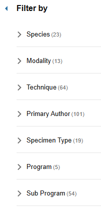
Scientists can filter for relevant projects across species, modality, technique, primary author, specimen type, program, and sub program.
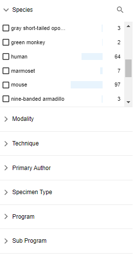
Click on the check box to apply a filter. The bars & numbers indicate the number of relevant result, e.g. 97 projects for species mouse. Numbers update relative to the selected filters.
Clear filters
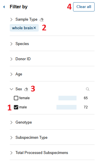
Scientists can clear
- individual filters by unchecking the checkbox in the extended section view
- clicking X on the filters chips in collapsed sections
- all filters in a specific section by clicking the eraser button
- all filter via the Clear all button
Browse Data Catalog
Program details pages
Large scientific consortia, e.g. NIH’s BRAIN Initiative Cell Census Network (BICCN) or BRAIN Initiative® Cell Atlas Network (BICAN), are distributed across many contributing organizations and generate a lot of important data.
The program pages in the BKP’s Data Catalog enable scientists to get an overview of these consortia and their available data at a glance. Example include BICAN and BICCN program pages.
They feature a short text introduction to the program:
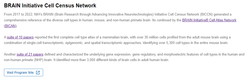
An interactive dashboard summarizing the available data. It allows scientists to access all projects from a given project in the BKP’s Data Catalog, e.g. 104 BICCN projects.

They can also click through to more granular search results, e.g. a search filtered to the 64 BICCN projects where the species is mouse.

Featured projects further highlight choice resources:
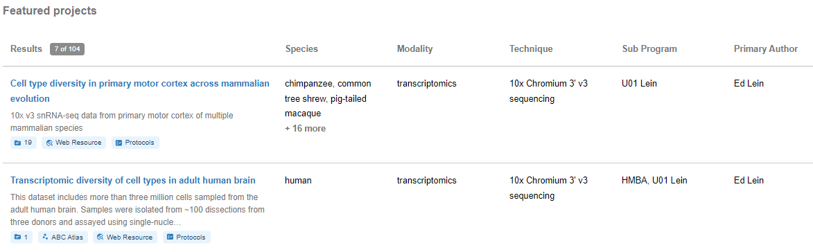
They feature core project metadata as well as preview indicators of data and resources associated with a given project:

Lastly, they include references to various related resources. These include landing pages, tools, protocols, data archives, and more.

Project details page
Project description & data overview
The top of the project details page features a text description summarizing the project. It also features an overview of the species, modalities, techniques, and specimen types involved.
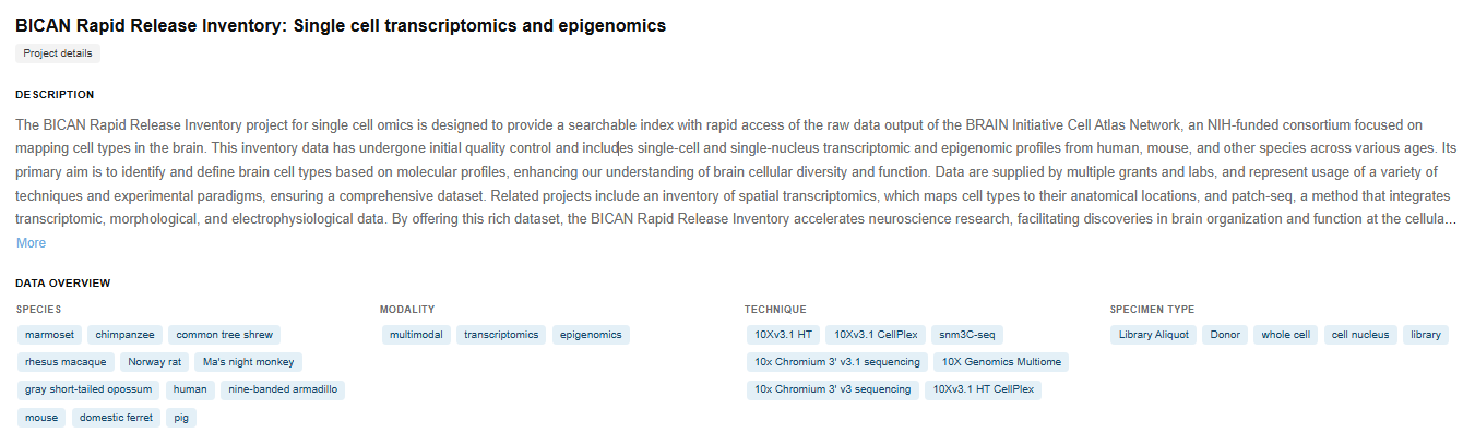
Other project metadata
A side panel offers additional project metadata, including detailed links to licenses, funding sources, and protocols.
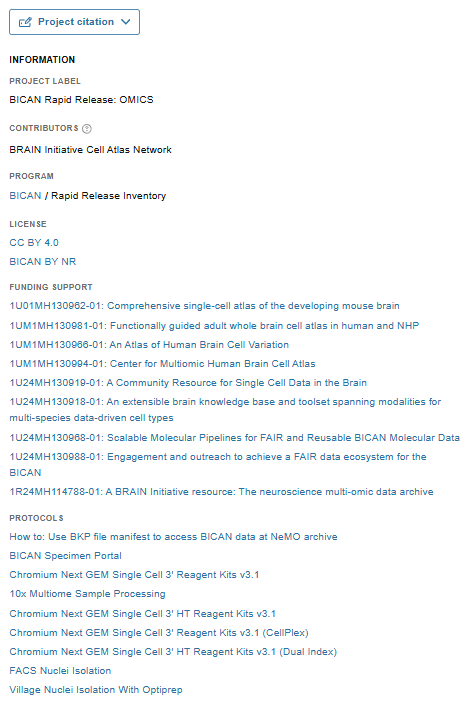
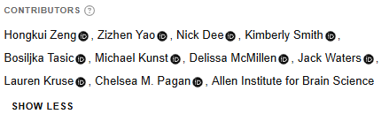
Note that if a project has both primary authors and general contributors, the primary authors are shown by default.

When the contributors are expanded, both primary author and general contributors are show.
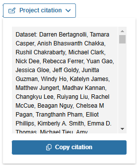
Citation button
Click the dropdown to view the citation.

Then click the “Copy citation” button to copy it to your clipboard.
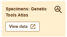
Highlighted resources
Click the buttons to access the highlighted resources. Project related resources can include:
Data visualizations, e.g. via ABC Atlas

Specimen metadata tables & their file manifest
Links to access raw or processed data files:
Other related resources, e.g. documentation:
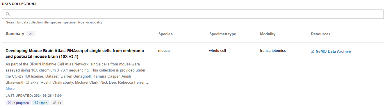
Data collections
A project’s data collections are listed at the bottom of the project details page. Scientists can see the total number of available data collections (20 in the example screenshot) as well as collection metadata:
- Name & description
- Species
- Specimen type
- Modality
- Resources, e.g. a link to an archive to access the files
- Last updated timestamp
- Status, e.g. in progress vs completed
- Accessibility: e.g. open vs restricted
- Number of specimens in the collection
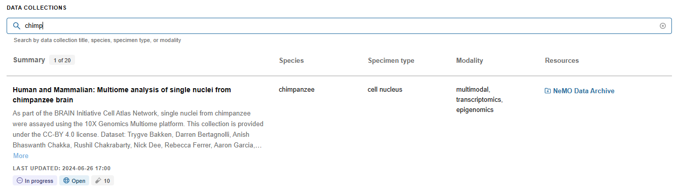
Scientist can text search across collection titles, species, specimen types, or modalities to find relevant collections quickly.
Note that when searching, the indicator changes to how many of the total collections match your query.
Remove the search by clicking the circled X in the search field.
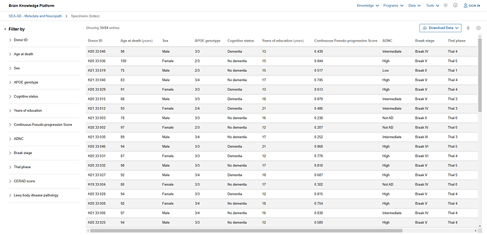
Specimen details page
Specimen table view
The filter menu is displayed to the left of the results table. It’s width is adjustable.
Collapse the filter menu by clicking on the "<" button. Expand it by clicking on the ">" button. Expand the individual filter sections and apply them by checking the desired boxes.
Numbers and bar graph visuals illustrate the number of matching results.
Clear filters individually or by clicking the Clear all button. See the faceted search section above for more details.
Column headers feature improved help text and column widths can be adjusted more easily. Hovering over table rows provides visual feedback.
Display properties controls
Display property controls represent selected vs. available content.
Text search across the properties saves time spent scrolling and enables scientists to find the right property quickly.
Selected display properties are indicated by a check mark and bolt font.
Note: If you hide a column that you’re actively filtering on, those filters will be removed.

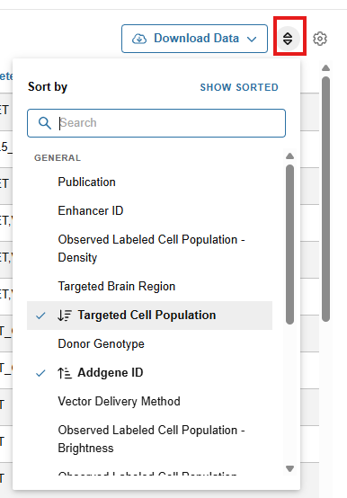
Sorting controls
Updated sorting controls more clearly represent selected vs. available options.
Text search across the properties saves time spent scrolling and enables scientists to find the right property quickly.
Selected sorting are indicated by bolt font. Icons represent ascending or descending order. Click on the icon to change sort order.
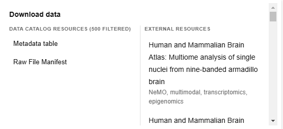
Metadata and file manifest download
Scientists can download metadata and file manifest for a set of specimen via a more prominent download button.

Metadata downloads match the filtered columns & rows in the UI. File manifest downloads match the specimen selection. Scientists can distinguish between downloads from Data Catalog and external archive resources in the popover:
Select individual rows for file manifest download
Projects that include a raw file manifest, allow scientists to select individual rows for their manifest download. This allows additional granularity beyond the filter panel.
Check the box at the beginning of the desired row(s) and then trigger the download.

Remove row selections individually.
Note: They also get removed when you clear all filters via the Clear all button.
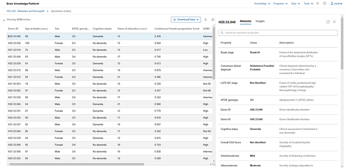
Side panel: specimen metadata
Click on a table row to open the specimen’s metadata details view in a side panel on the right. Note that the row remains highlighted in the table. The metadata details view features all metadata for a given specimen and goes beyond the chosen display defaults. It allows scientists to get the gist for any given specimen. Scientists can quickly find the relevant to them metadata field via test search across the metadata properties, values, and description.
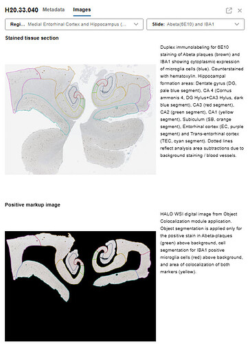
Side panel: image viewing
When available, this is the default loaded state of the side panel. The side info panel includes access to relevant imaging data, e.g. neuropathology or epifluorescence.
The image viewing will feature at least one of the following solutions:
- an integrated image view with dropdowns to select your image of choice
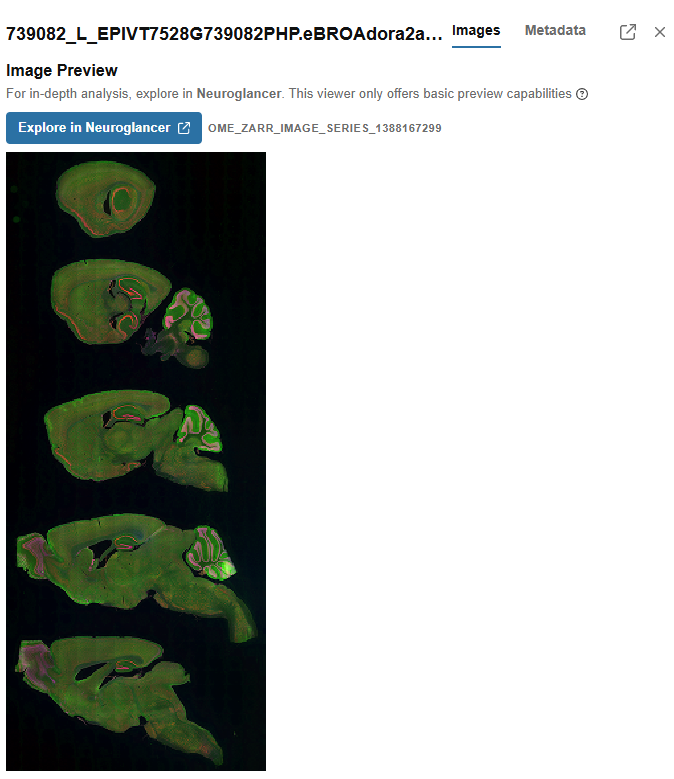
- a preview of the available images
- a link to open the image in a dedicated image viewer in a new tab
Note: Neuroglancer previews are interactive. Scroll with your mouse wheel to flip through the image slides. Use Ctrl + Scroll to zoom in on the image location your mouse curser is pointed.
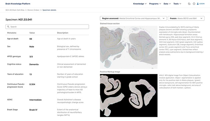
Specimen details view
In the side info panel, click on the following icon to open the specimen details view:

It opens a new tab that features the above specimen metadata and image viewing tabs side by side.
Breadcrumbs allow scientists to navigate within the current project.
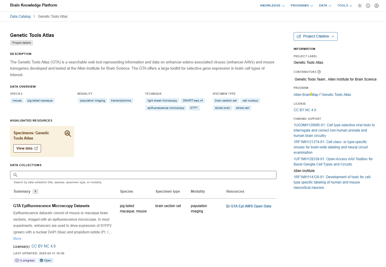
Explore the Genetic Tools Atlas to find AAV vectors and transgenic lines. Select optimal genetic tools for your cell-type specific research.
The Genetic Tools Atlas (GTA) is a searchable web tool representing information and data on enhancer-adeno-associated viruses (enhancer AAVs) and mouse transgenes developed and tested at the Allen Institute for Brain Science. The GTA offers a large genetic toolkit for selective gene expression in brain cell types of interest.
Project Details page
View project metadata
Review the project metadata and linked resources on the project details page.
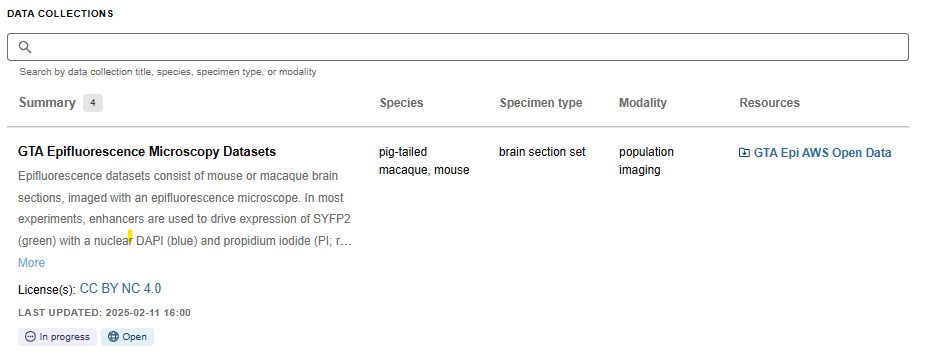
Search Collections
Search the available data collections and download files via the links in the Resources tab.
Access experiments
Access the experiment inventory.
Experiment inventory
Browse
Browse the experiment metadata, view expression imaging data, and download artifacts for downstream analysis.
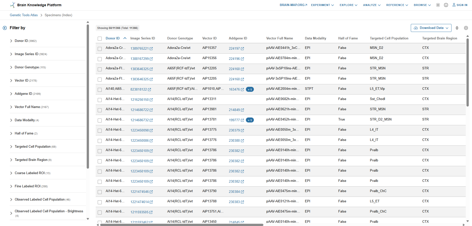
Adjust displayed columns
Click on the gear icon and select or unselect columns to customize your view. Filter options and filter order will automatically match the displayed columns
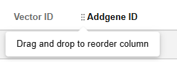
Note: You can adjust the column order by dragging & dropping a column in the table. Click on the handle next to the column header and drag it to it's now position.
Sorting columns
Click on a column header for simple sorts on a column in ascending or descending order.
For multiple sorts, use the sort controls.
Filter columns
Set filter
Each column can be filtered via faceted search filters. Expand a filter and search for your facet of interest by scrolling or using text search via the loupe icon. Then select your filter of choice by clicking the checkbox. The number of entries for a given filter are indicated on the right.
Note: Selecting on one filter category, will update the available options in order filter categories.
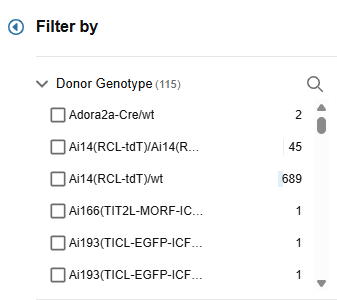
Remove filter
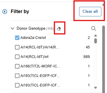
Filters can be removed:
- individually - uncheck the checkbox
- by category - click the eraser button
- overall - click the Clear all button
View side panel
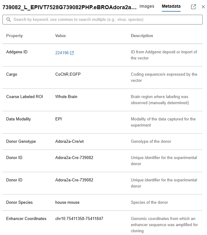
Click on a table row to open the side panel. It features two tabs: Images & Metadata.
Images is the default load behavior. More on viewing images below.
The metadata section shows all metadata columns and entries for this selected entry, even ones, that are currently not selected in display column. Use text search to search the metadata.
View images
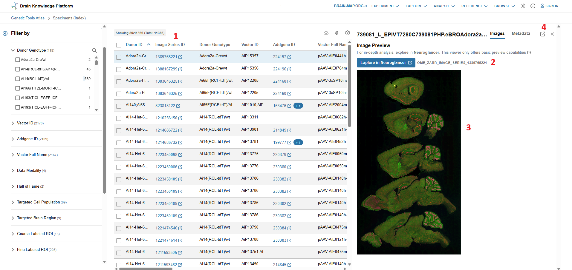
View the expression images associated with a given experiment by:
- Opening the image in Neuroglancer by clicking on the Image Series ID in the table
- Click on a table row and then click on the Neuroglancer button in the preview side panel
- Click on the table row and observe a preview of the image preview in the side panel
- Open an experiment details page that displays all experiment metadata and the image side-by-side
Download artifacts
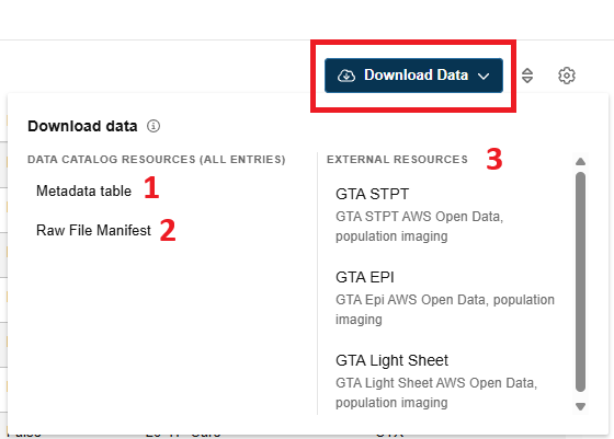
Download the:
- metadata table
- raw file manifest
- external resources
Master the ABC Atlas platform with our complete user guide. Learn to navigate cell type taxonomies and explore molecular data across the whole brain.
The ABC Atlas aims to empower researchers worldwide to explore and analyze multiple whole-brain datasets simultaneously. As the Allen Institute and its collaborators continue to add new modalities, species, and insights to the ABC Atlas, this groundbreaking platform will keep growing, opening up endless possibilities for groundbreaking discoveries and breakthroughs in neuroscience. With the ABC Atlas, researchers everywhere can gain new insights into the brain’s complex workings, advancing our understanding of this amazing organ in ways we never thought possible.
In addition to incorporating new data regularly, the ABC Atlas will continue to be updated every few weeks with new features and capabilities. Please let us know what you like, what you don’t like, and what you’d like to see in future updates!
Overview
The icon panel on the left allows quick navigation between Control Panel tabs. The filters and settings on each tab all work together to change what is displayed in the visualization frames to the right.
There are three tabs, each controlling a different aspect of the visualizations:
- Manage Layouts - Find data to add to your view or change your layout
- Cell Properties - Filter and color by data features and values
- Genes - Search, select, and color by gene expression
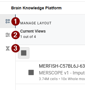
Manage Layouts & Browse Data Sets
The Manage Layout tab allows adding, changing, and reordering visualization frames. Frame settings like point size and transparency can also be accessed here.

Adding and changing views
- To add a new visualization click the + icon in an open row.
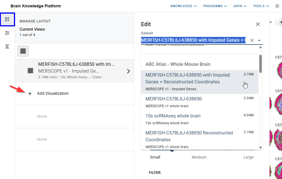
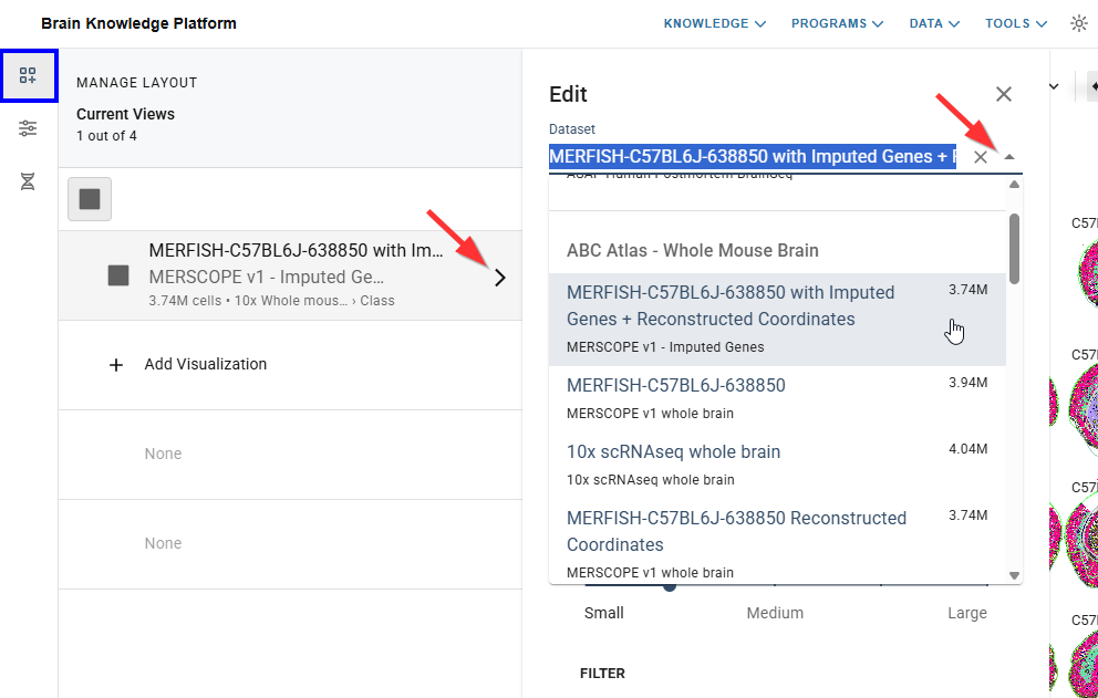
- When adding or changing a view, the data set can be selected using the dropdown list in the pop-out menu
- The layout orientation can be changed by clicking the icons at the top of the panel. Change the order of views by dragging and dropping a row in the list.
Settings
Resolution/Performance
The balance between resolution quality and rendering speed may be adjusted using the Resolution/Performance slider in the Settings tab. In order to dynamically render the millions of points in our data sets, we use a sophisticated sampling algorithm that trades off speed for resolution when zoomed out. Depending on system set up, the data being viewed, and exploration goals, the slider may be used to increase speed and reduce resolution or vice versa.
The same setting may produce different results with different data sets or different system setups. We encourage you to experiment with the settings to find the one that works best for your needs
Please note:
Your device, internet connection, browser, and other factors can influence performance and loading speed. For best results, we recommend using the ABC Atlas in an updated version of the Chrome browser and closing unnecessary programs and browser tabs. If you experience significant performance issues, please let us know using the feedback survey and include your system details.
Point Size
The size of the points (cells) in the visualization frame can be changed in the Settings tab. Move the Point Size slider to the left for smaller points (for less overlap) or to the right for larger points (for denser visualizations). Points will dynamically resize as you zoom in or out relative to the size selected.
Transparency
- If a filter has been applied to your visualization, you may adjust the prominence of the unselected cells.
- To change transparency, navigate to the Settings tab within the Control Panel and click the checkbox and adjust the slider to change the opacity.
- Setting the transparency to the lowest level will remove the unselected cells completely.
Cell Properties
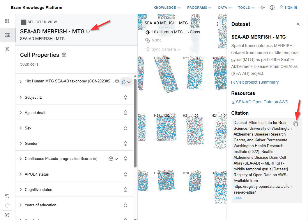
To learn more about the selected data set including download links, sharing, and citation tools, click the (i) icon next to the data set name.
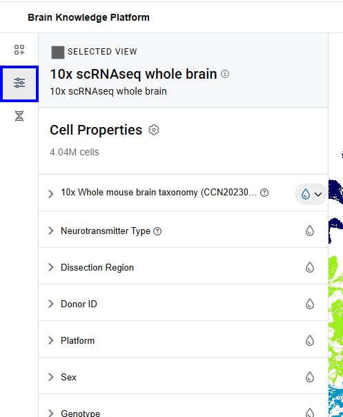
Color
- You may apply color to your visualizations to help distinguish cells within a category or gene expression.
- Color values are predetermined and may only be applied to one feature at a time.
- Click the droplet icon to the right of a feature to color by that feature. The currently colored feature is indicated by a gray circle highlighting its droplet.
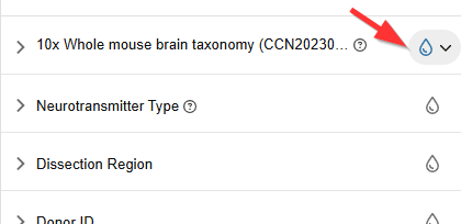
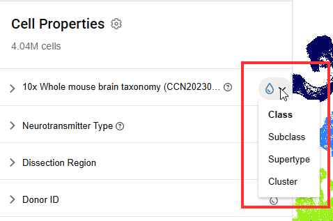
- For hierarchically nested features, the droplet will have a small arrow to the left. Click the arrow to display a dropdown menu with additional coloring options.
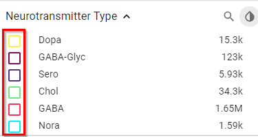
- If color has been selected for a feature, the checkbox next to its sub-values will change to reflect each value’s corresponding color in the active frame.
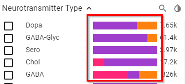
- When you color by a feature, values under the other features show the distribution of cells in the next lower level of the hierarchy as a horizontal bar next to that value. When a filter is applied, only the selected values(s) will display this bar.
Filtering
- Color may be applied to a subset of cells in the visualization using filters.
- Multiple filter selections within a feature will include any cells that meet either criterion (OR), while multiple filter selections across features will only display cells meeting all criteria (AND).
- When no filters are selected, the total number of applicable cells appears next each value within a feature. Once a filter has been applied, only the selected values will show cell counts, other unselected values will display zero.
- To filter cells from your active frame, check the box next to a value you wish to see colored. Cells with any other value within the feature will be grayed out. See notes on Transparency to adjust the opacity of these filtered-out cells.
- When filters have been applied, a gray badge appears at the top of the feature section indicating the number of active filters. To remove all selected filters, click the “x” in the gray badge.
Genes
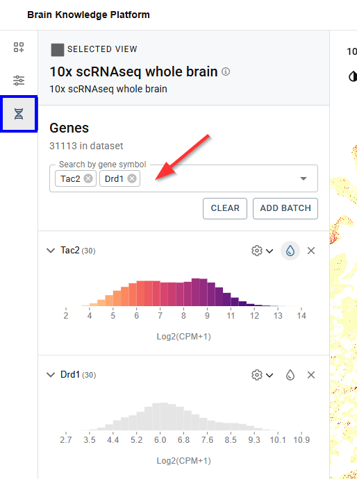
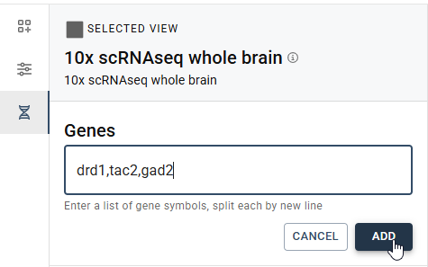
On the Genes tab, search and select multiple genes in the search bar or use the Add Batch button to add a list of genes all at once.
Gene Expression Settings
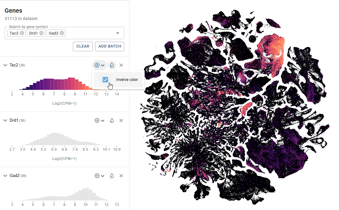
To invert the color map, click the gear icon and check the “Inverse color” box.
Gene Expression Filtering
To filter views by gene expression value, from the Genes tab, after selecting a gene, click on the gene name to show the expression histogram. Click anywhere in the histogram to initiate filtering, then click and drag the vertical bars to adjust the values shown in your filter. Only one numeric feature filter is allowed at a time. To remove the filter, click the eraser icon to the right of the gene name.
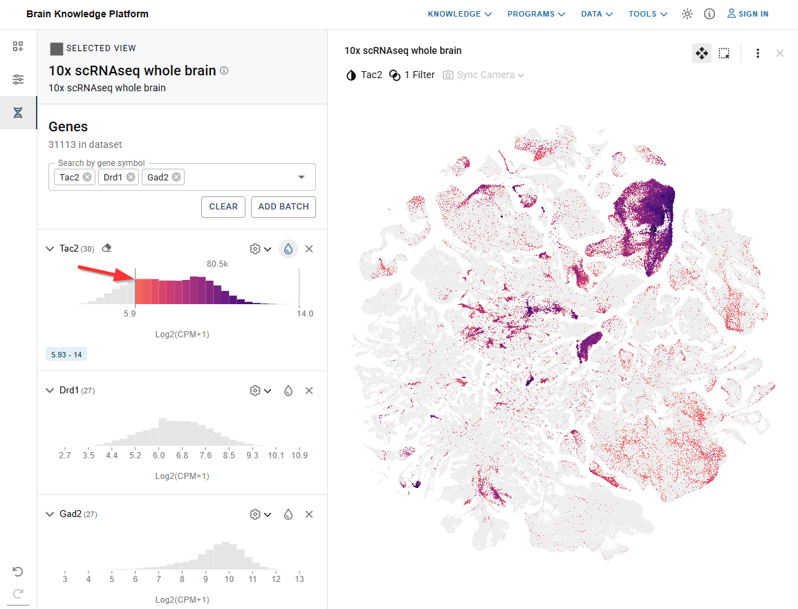
Tip: You can filter by gene expression values while coloring by a different feature, including other genes.
Share and Citation
Share
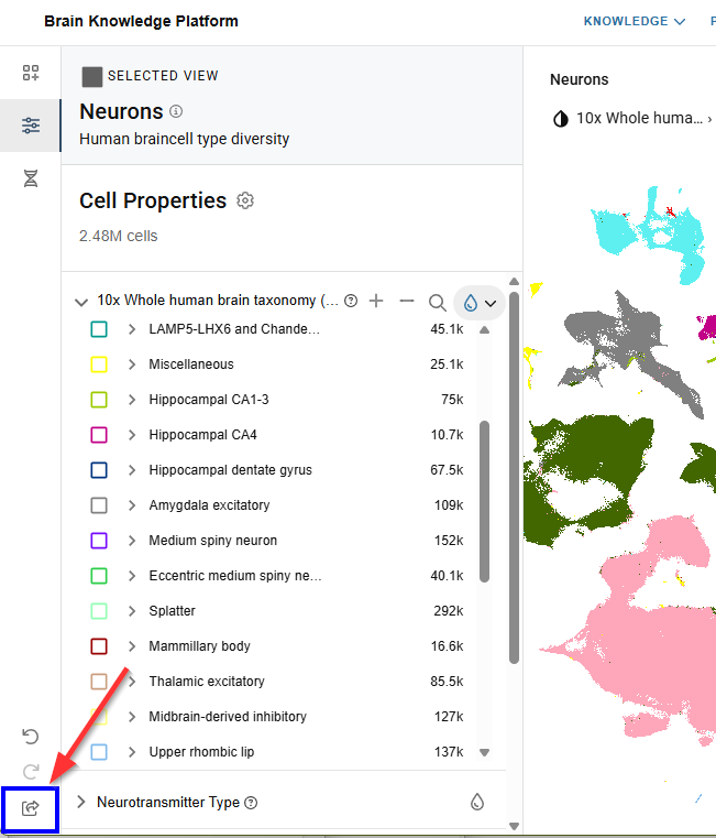
Click the icon in the lower left to copy a link to the current set of visualizations. The link saves the state of all views including, filters, colors, and camera positions and can be shared with others or saved for future reference.
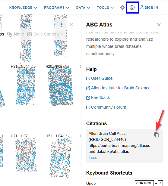
Project Citation & ABC Atlas Tool Citation
To cite the ABC Atlas tool click the info icon in the top navigation bar then click the copy icon under Citations in the right panel.
To cite the data displayed in ABC Atlas click the Dataset info icon then the copy icon under Citation in the right panel.
Visualization Frame
The ABC Atlas allows you to view up to four visualizations at the same time. When viewing multiple visualizations, the active frame is indicated by a bold outline. Only the active frame will be affected by selections made in the Control Panel.

Tool tips
Hovering your mouse over a cell will display details of the cell’s color. For example, if your visualization is colored by Class, hovering over a cell will show which class the cell belongs to. If multiple cells overlap, the most common cell in the area will be shown.
If the data supports anatomical overlay, the tool tip will also show which anatomical area the cell is in.

Hover Sync
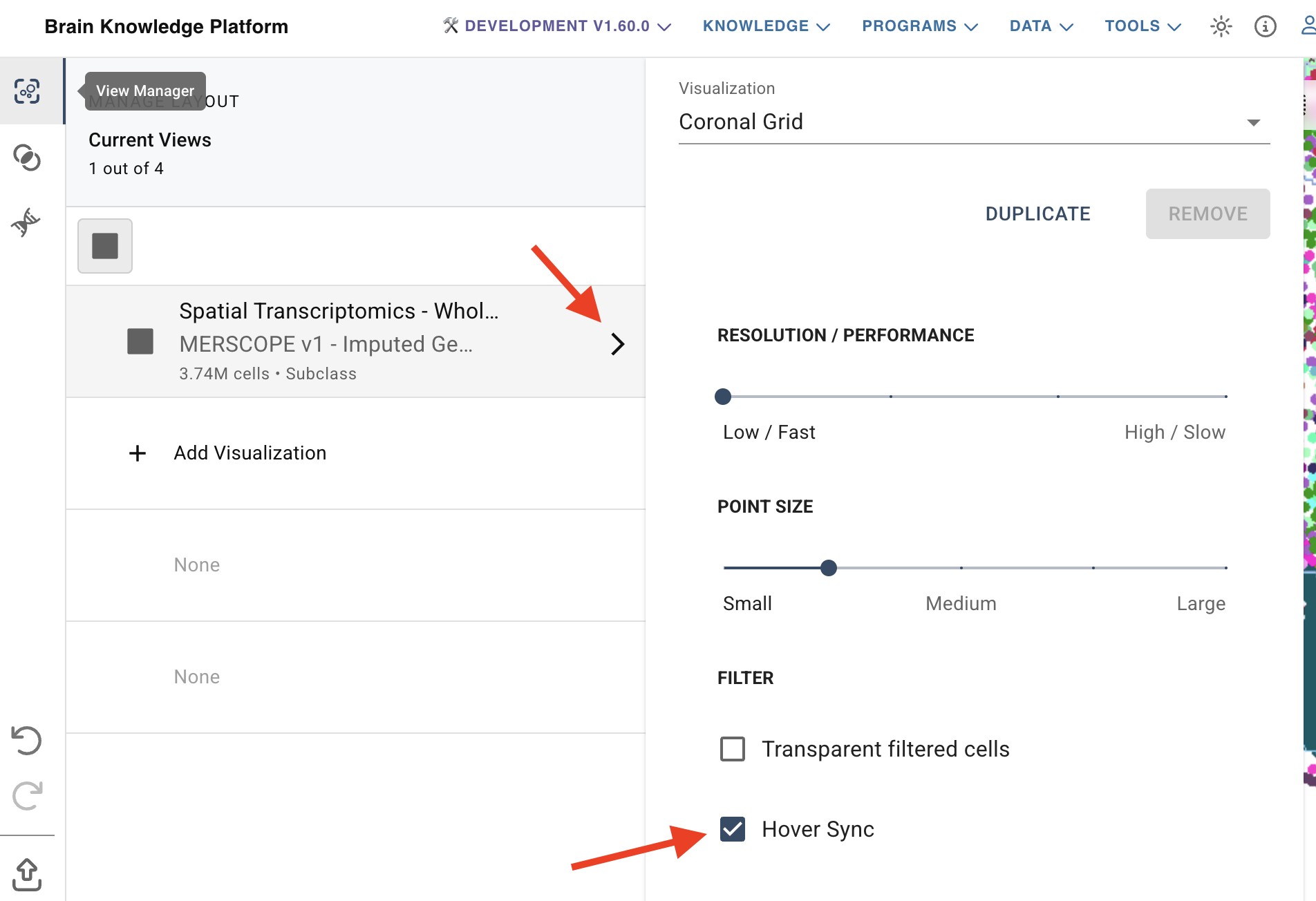
The “hover sync” is a feature that allows you to quickly see and compare cell property values which are shared across data sets.
When hovering over a cell in addition to the cell property displayed in the tool tip, other cells in the view temporarily increase in size to show where else that value occurs. If other views are open with cells that share that value, those cells will also temporarily increase in size.
For example, when viewing the Zeng and Zhuang whole mouse brain data sets side by side and coloring by cell type in both views, hovering over a cell type in one view will highlight the same value in the other view.
This same cross-view highlighting can also be achieved by hovering over a value in the cell properties left tool bar.
To turn this feature off for the selected view, uncheck the Hover Sync box in the settings.
Duplicate View
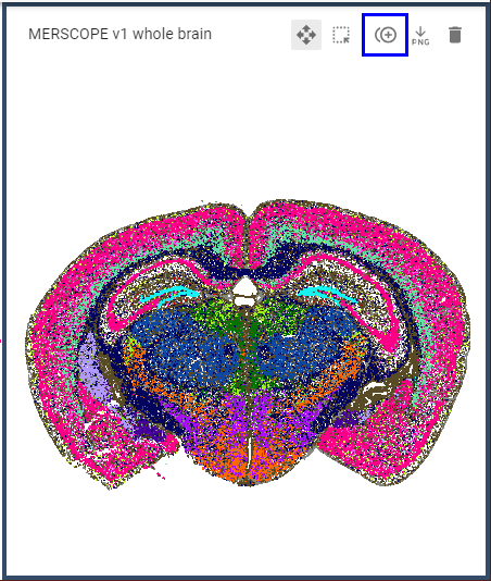
In the top right of the selected view, clicking the third icon from the left will create a new view with the same colors, filters, pan, and zoom settings as the active view.
Download image
This creates a high-resolution PNG image of the selected view and initiates the download through your browser.
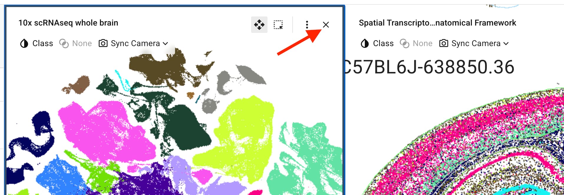
Close
Click the X in the upper right of the active frame to remove it from your layout.
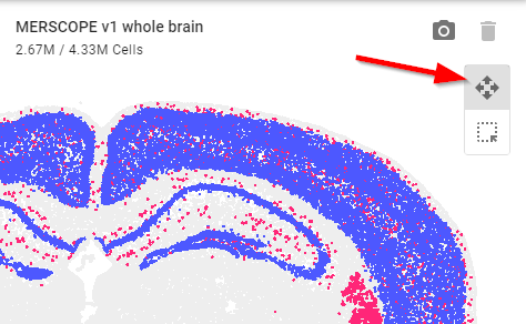
Navigation modes
- ABC Atlas allows two navigation modes, Zoom & Pan or Cell Selection. The active navigation mode is indicated by and can be changed using the icons in the top right of the active frame. Only one navigation mode is active at a time.
- Zoom & Pan is indicated by four arrows and Cell Selection is indicated by the perforated square.
Camera Controls (Zoom & Pan)
- Use your mouse scroll wheel to zoom in to view more detail or out to see more of the visualization at once.
- Click and drag to view a different area of the visualization.
Camera Syncing
Camera Syncing creates spatial sync groups between views of the same data set, allowing you to control two or more views at once. When syncing is enabled, as you zoom in or move the “camera” in one view, synced views will follow, maintaining the same position. Syncing does not affect selected filters or colors so that you can compare different features in each view.
- To initiate Camera Syncing, click Sync Camera in the top right of the selected view.
- Check the box next to the view you’d like to sync with.
Now any change made to the zoom or pan state in one view will also be reflected in the other view.
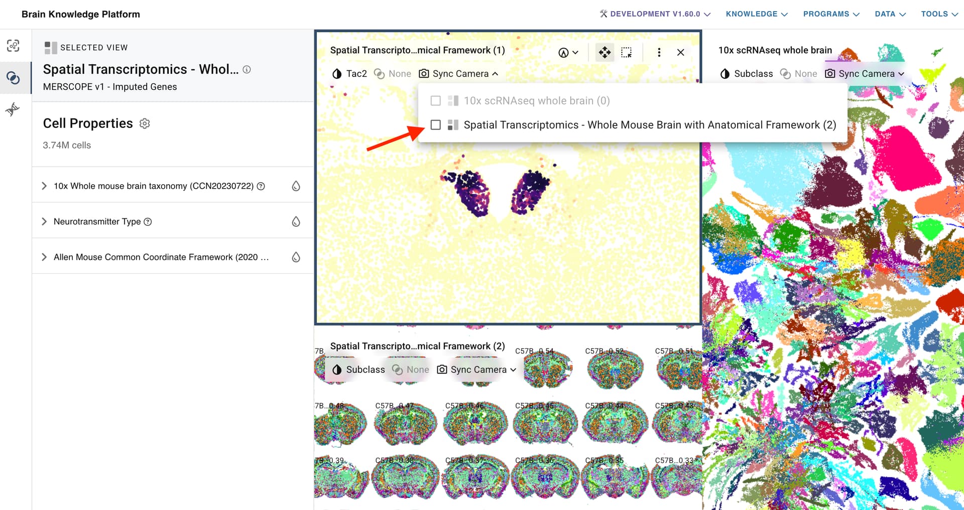
Enabling syncing for additional views of the same data will add them to the original sync group. Note: Only one sync group per data set is supported.
- Unselect the checkbox to remove a view from the sync group and allow the camera for that view to be controlled independently.
Slide View
Data sets comprised of spatial slices of tissue offer additional viewing options including the ability to scroll through slices while maintaining zoom and pan positioning.
- Advance through slices in order using any one of the following mechanisms:
- use the arrow buttons at the top of the view
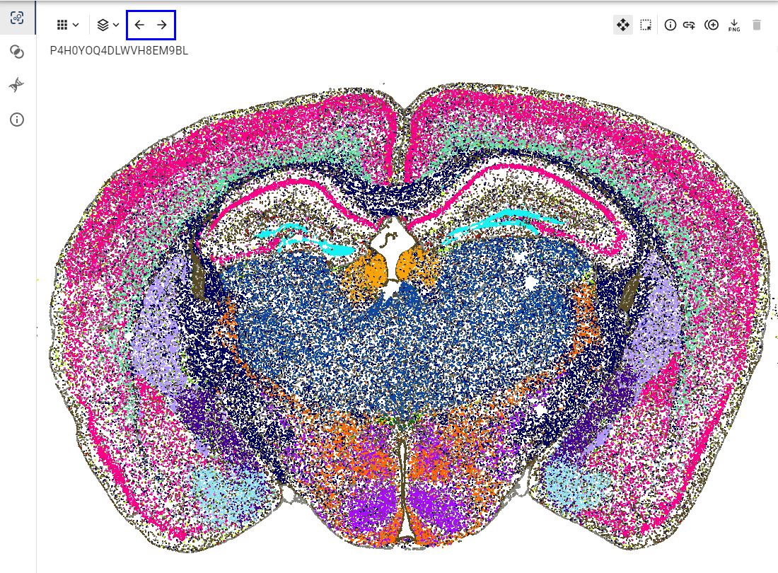
- simultaneously hold the Alt key on Windows (Option key on Mac) and scroll the mouse wheel
- hold the Alt key on Windows (Option key on Mac) and press the arrow keys
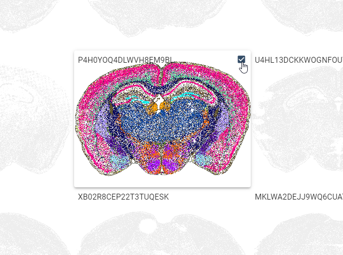
- Show or hide specific slices to create a custom view by checking the box in the upper right hand corner of each slide to be shown.
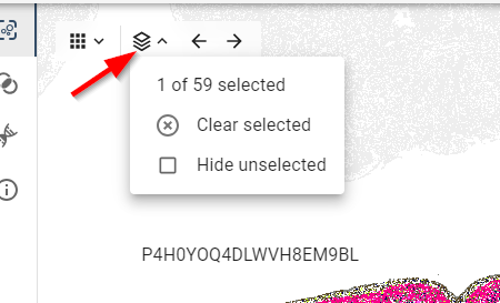
- To completely hide unselected slices, click “Hide unselected” from slide menu in the top left of the view.
- Pick “Clear selected” from the slide menu in the top left of the view to clear all selections or uncheck all boxes.
Cell Selection
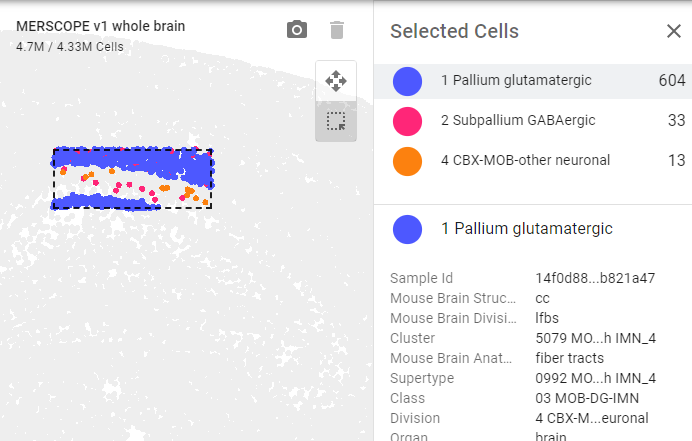
- In Cell Selection mode, click and drag to highlight cells in a specific region of the visualization to open the Selected Cells panel.
- Once cells have been selected, the top portion of the Selected Cells panel displays an aggregated view of the cells in your cell selection region grouped by your current color selection.
- The bottom portion displays the details of each cell in the highlighted aggregation group. Click on a different aggregation group in the top section to switch groups.
- Press the shift key once to enter Cell Selection mode. Press shift again to exit.
- Zoom & pan controls will continue to work even when in Cell Selection mode. Use the scroll wheel to zoom and hold the space bar to pan.
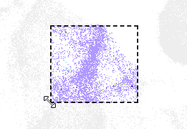
- When in Cell Selection mode, the selection box can be resized by hovering over the edge until the cursor becomes a double-sided arrow and then clicking and dragging to the desired size.
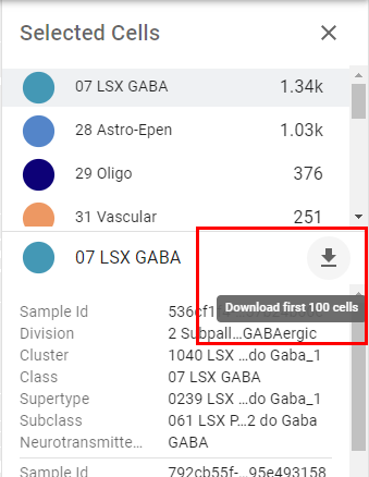
- While in the Cell Selection view, details of the selected cells can be downloaded as a csv file. Please note, only the first 100 cells will be included in the download. Full dataset download is available via GitHub .
- Use the Zoom and Pan mode to focus in on the desired region of cells
- Switch to Cell Selection mode and drag to select a specific set of cells
- In the Selected Cells list, click on a aggregation group value
- Click the arrow icon to initiate the download
Header
Light/Dark Mode - Toggle between light and dark color scheme by clicking the moon icon.

Help - Access information about the ABC Atlas including documentation, our community forum, and provide feedback and suggestions to help us improve your experience.

Give us your feedback and suggest new features here: Allen Institute - Feedback
Master Allen Brain Explorer desktop application for 3D visualization. Navigate brain atlases, view gene expression, and create custom visualizations.
Brain Explorer® 3D Viewer is an application for viewing brain anatomy and gene expression data in three dimensions in the framework of the Allen Developing Mouse Brain Reference Atlas.
Using Brain Explorer, you can:
- View fully interactive versions of the Allen Developing Mouse Reference Atlases in 3-D.
- View gene expression data in 3-D at 200 µm 3 resolution.
- View expression data from multiple genes superimposed on each other in 3-D.
- Navigate the high-resolution 2-D ISH images using the 3-D model.
- Link to associated gene metadata on the Allen Developing Mouse Brain Atlas web application.
Installation
Windows
Systems requirement: minimum configuration
- Operating System: Microsoft Windows 7
- CPU: Intel Core Duo or AMD 1.8GHz
- System Memory: 1GB
- Graphics Card: Hardware 3D OpenGL accelerated AGP or PCI Express with 64MB RAM
- Screen: 1024x768, 32-bit true color
- Hard Disk: 200MB free space
Note: Brain Explorer is known to work with the following video chipsets: nVidia GeForce 9400/9600, nVidia Quadro FX 1800/3800/5600, AMD Radeon 9600, AMD Radeon HD 3200/4550, Intel Q35/Q45 Express.
For the best performance, please check with your video card vendor for the latest available drivers before using Brain Explorer. The Windows version of the Brain Explorer viewer is available here. Double-click the downloaded BrainExplorer2.msi file and follow the prompts.
Mac
Systems requirement: minimum configuration
- Operating System: OS X 10.6.8
- CPU: Intel 1.8GHz
- System Memory: 1GB
- Graphics Card: 3D-capable with 64MB RAM
- Screen: 1024x768, 32-bit millions of colors
- Hard Disk: 200MB free space
Note: Please install the latest system updates from Apple to ensure you have the latest video card drivers.
The Mac version of the Brain Explorer viewer is available here. Double-click the downloaded zip file to unpack Brain Explorer.
Installing Atlases
A one-time download containing anatomy files is needed following installation of the Brain Explorer application. The first time you open the Brain Explorer software, you will be asked to choose to download files for the Allen Mouse and Allen Human Brain atlases. Click on the atlases you would like to use and then click the Install button.
To download missing atlases on the PC, go to the Help menu and select Download Atlases. On the Mac, the command is in the Brain Explorer 2 menu.
Getting Updates
The Brain Explorer application will inform you when updates to the Brain Explorer application itself or its atlases are available. New data may not be available for viewing until you install the required updates.
Viewing Gene Expression
To load gene expression data into the Brain Explorer viewer: go to the Allen Developing Mouse Brain Atlas and perform a search. Your search brings back a list of genes that fit your search criteria. Click on a gene name to select a gene of interest. 3-D thumbnails at all developmental stages of the gene expression pattern from that gene will load to the right. Click on the blue “View in 3D” link to launch the Brain Explorer application and load each experiment.
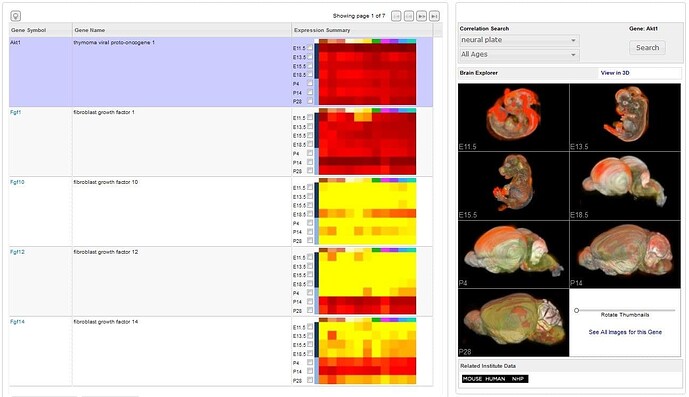
When the Brain Explorer 3-D Viewer opens, you will be taken to a screen that displays the Image Viewer, the Structure Ontology Viewer, and the Gene List.

Image Viewer
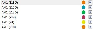
The Image Viewer will display the gene expression representations in 3-D for your gene of interest across all stages. Each stage will default to separate color schemes for each developing stage. For each developing stage, a sphere represents expression re-sampled to a grid resolution that is dependent on the stage in question (see the Informatics Data Processing whitepaper available in the Documentation. Larger spheres correspond to a greater density of expression in that voxel.
You can filter the developmental stages by hovering your mouse over the age to bring up an “X” or a magnifying glass. Clicking on the “X” will close that experiment, clicking on the magnifying glass will remove all the other stages from the viewer.
You can select a sphere by clicking on it. Spheres can be deselected by clicking on blank space. The original ISH image of the selected sphere will be displayed blended with the expression heat mask in the lower left-hand portion of the screen. The blending can be adjusted by selecting Image Controls from the View menu and moving the Image Blending slider. Clicking on the arrow in the top right-hand corner of the zoomed ISH image will open the corresponding ISH image in a high resolution image viewer.
The information at the upper-left corner of the main Brain Explorer window summarizes the expression detected in the selected grid location. These numbers include the average expression density and intensity (over pixels). The Informatics Data Processing White Paper describes how the measurements were obtained.
To change the gene expression representation, click on the “Data” menu and select an option under “Raw” colors.
A compass in the right-hand corner of the Image Viewer can be used to rotate the brain(s) by clicking and dragging your cursor. You can zoom using either the wheel on your mouse or using the Zoom scrollbar in the lower right-hand corner of the Image Viewer.
Expression Thresholds
A way to control expression visibility is by setting thresholds on expression values. This method can restrict visible spheres to different combinations such as low intensity and low density or high intensity and low density.
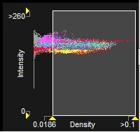
The graph in the lower right-hand corner shows a dot for each data point (sphere) in a gene expression file, and the color of the dot corresponds to the anatomic annotation in the same way the atlas colors display mode works. Each data point is plotted according to its density on the x-axis and its intensity on the y-axis.
The color scale on the left-hand side of the graph corresponds to the expression level heat map used to color the spheres, color coded to the reference atlas structures. The numbers along each axis show the values at the yellow triangles.
The thresholds can be changed by resizing the white box. Any edge or corner of the box can be clicked and dragged to re-size it. You can also click and drag in the center of the box to move the box.
Structure Ontology Viewer
The Structure Ontology Viewer shows the entire collapsible ontology for the developing mouse brain as defined by the Allen Developing Mouse Reference Atlas. The first column represents the color of the reference atlas for that structure. The two columns to the right determine the type of data displayed in the Image Viewer. “A” represents atlas structure and when checked, will show a visual representation of that structure in the Image Viewer. “D” represents gene expression and when checked, will show gene expression in that structural domain.
The default organization for the Structure Ontology is the Hierarchical View, but if you are unfamiliar with the ontology, you can click on the Alphabetical View to see the structure list in alphabetical order.
The Bookmarks tab is a space where you can create and save favorite views of the brain. Several default views are already saved that will rotate the brain back into common viewing frames.

Gene List
This section displays the experiments you have selected and downloaded in this session. Right clicking on the gene name will bring up a menu where you can, 1) view the gene detail page (Get Info), 2) be taken to a zoomed in image from this experiment (View Images), 3) copy meta information to the clipboard, such as symbol, name, Entrez ID, image-series ID (Copy Info), 4) activate a Correlation search by finding experiments with similar expression profiles (Find Similar) or 5) close the experiment and remove it from the list and the 3-D view (Close).
Gene Search
To search for genes within the Brain Explorer application, go to the Search box located above the ontology panel and type in the gene symbol or part of a gene name.
The list of results shows gene name, gene symbol along with a 3-D summary thumbnail of the expression for each experiment matching the search. The expression thumbnail represents a maximum expression projection rendering: the denser the expression in a region the more “solid” the appearance. Reference atlas colors are additionally layered on top.
To load an experiment for viewing, click on the “Download” button under the gene name.
Toolbar
| Button | Operation |
|---|---|
 | Selects cursor rotation tool mode |
 | Selects cursor pan tool mode |
 | Selects cursor selection tool mode |
 | Toggle Sagittal Atlas section viewing |
 | Toggle Coronal Atlas section viewing |
 | Toggle Horizontal Atlas section viewing |
 | Centers the Viewer on the current pinpointed expression data point |
 | Turns on the cutting planes |
 | Toggles the Structure Ontology and Gene List View |
Advanced Features
Atlas Menu:
You can show opaque three dimensional structures of the brain by “showing” or “hiding” structures from this menu. The “Transparent” function allows you to see transparent views of the structures to view the anatomical relationships between them.
Selecting the sagittal, coronal or horizontal sections (or clicking on one of the section image buttons in the toolbar) will superimpose a single plane of the reference images (Nissl or Feulgen-HP) from each brain on your image space. These planes can be moved once the selection tool mode button in the toolbar is selected. Selecting “Show Annotation on Section” from this menu will color the reference images according to the brain structure ontology.
Data Menu:
When you have a gene selected, the Data menu allows you to show all expression, hide all expression (for instance to then select a single structure) or toggle expression (for instance, unselect your region of interest then toggle to see expression in only that region).
You can also show or remove threshold controls and choose the visual representation of your data from this menu. There are several options under “Raw” colors:
- User defined: Each experiment is rendered in user specified color. This mode is useful to distinguish between individual experiments when multiple experiments are being displayed.
- Atlas: In this mode the sphere is colored by the corresponding reference atlas structure color. This mode is useful for quickly seeing the annotated regions where a gene is expressing.
- Signal Level: This mode displays average expression intensity and is useful for identifying areas of very high expression.
- Jet: Applies the common “jet” colormap to the data.
To be taken to the experimental detail page, select “Get Info”. To see a high resolution image view of this experiment, choose “View Images”. These functions are also available by right-clicking on the gene name in the Gene List.
Choose “Find Similar” to find similar genes to the selected experiment. This uses the same Correlation Search functionality as in the web application.
Clipping Planes:
When this function is selected, either by toggling the cutting tools button in the toolbar or selecting “Clipping Planes” from the View drop down menu, you can make coronal, sagittal or horizontal cuts in your view of the brain and related data. To cut in a particular plane, make sure the cursor is in selection tool mode, and then click and drag on the plane you are interested in clipping.
Troubleshooting
Windows
Graphics
If you are using a desktop computer, you should obtain drivers from the video card manufacturer. First, identify the video card. Go the Start menu and open the Control Panel. Open the Display control panel and go to the Settings tab. Click the Advanced button and go to the Adapter tab. Your video card vendor and model name will be displayed at the top of the window under Adapter Type. Please go to the manufacturer’s web site, locate the driver download, and follow the instructions on the website or included with the downloaded file.
If you are using a laptop computer, you will need to go to your laptop manufacturer’s web site to locate the latest video drivers.
You can also activate an alternate drawing mode in Brain Explorer. Go to the View menu and select Options. Check the Draw faster but at lower quality button and uncheck the Synchronize drawing with the monitor’s vertical refresh button. Set the Multisample setting to Off.
If you are using multiple video cards from different vendors, the 3-D display may not work correctly on all attached monitors.
Uninstalling
Use the Add/Remove Programs control panel or the uninstall link in the Brain Explorer folder in the Start menu. Additional data that are not automatically uninstalled are located at the following locations:
Windows XP
Atlas data: C:\Documents and Settings\userid\Local Settings\Application Data\Allen Institute\Brain Explorer 2
User settings: C:\Documents and Settings\userid\Application Data\Allen Institute\Brain Explorer 2
Windows Vista and Windows 7
Atlas data: C:\Users\userid\AppData\Local\Allen Institute\Brain Explorer 2
User settings: C:\Users\userid\AppData\Roaming\Allen Institute\Brain Explorer 2
Proxy Settings
If you use a proxy server, the Brain Explorer application will use the proxy settings from the Internet Options control panel in the Windows Start menu. Please refer to the Windows documentation for help on proxy settings.
Mac
Uninstalling
Drag the Brain Explorer 2 icon to the trash. The Brain Explorer application generates the following files, which can also be dragged to the trash.
- ~/Library/Application Support/Brain Explorer 2
- ~/Library/Preferences/org.alleninstitute.BrainExplorer2.plist
Performance
If the Brain Explorer application is not running smoothly, first try to free up as much memory as possible by quitting all other open applications. You can also activate an alternate drawing mode. Go to the Brain Explorer 2 menu and select Preferences. Check the Draw faster but at lower quality button and uncheck the Synchronize drawing with the monitor’s vertical refresh button. Set Multisampling to Off.

Learn about Connected Services and Pipes with comprehensive guides and examples from Allen Institute for Brain Science.
service::dev_human_correlation
Parameters
Examples
http://api.brain-map.org/api/v2/data/query.xml?criteria= service::dev_human_correlation[set$eqrna_seq_genes][probes$eq1090294][structures$eq'CBC']
http://api.brain-map.org/api/v2/data/query.xml?criteria= service::dev_human_correlation[set$eqrna_seq_exons][probes$eq279330730][structures$eq'CBC']
Retrieve exon_microarray_genes correlation values for structure with the acronym, "CBC".
http://api.brain-map.org/api/v2/data/query.xml?criteria= service::dev_human_correlation[set$eqexon_microarray_genes][probes$eq9463][structures$eq'CBC']
http://api.brain-map.org/api/v2/data/query.xml?criteria= service::dev_human_correlation[set$eqexon_microarray_exons][probes$eq280550735][structures$eq'CBC']
service::dev_human_differential
Parameters
Examples
http://api.brain-map.org/api/v2/data/query.xml?criteria= service::dev_human_differential[set$eq'rna_seq_genes'][structures1$eqDFC][structures2$eqMFC]
http://api.brain-map.org/api/v2/data/query.xml?criteria= service::dev_human_differential[set$eq'rna_seq_genes'][structures1$eqDFC][structures2$eqMFC]
http://api.brain-map.org/api/v2/data/query.xml?criteria= service::dev_human_differential[set$eq'exon_microarray_exons'][structures1$eqDFC][structures2$eqMFC]
http://api.brain-map.org/api/v2/data/query.xml?criteria= service::dev_human_differential[set$eq'exon_microarray_genes'][structures1$eqDFC][structures2$eqMFC]
service::dev_human_expression
Parameters
Examples
http://api.brain-map.org/api/v2/data/query.xml?criteria= service::dev_human_expression[set$eq'rna_seq_genes'][probes$eq1090294]
http://api.brain-map.org/api/v2/data/query.xml?criteria= service::dev_human_expression[set$eq'rna_seq_exons'][probes$eq279330730]
http://api.brain-map.org/api/v2/data/query.xml?criteria= service::dev_human_expression[set$eq'exon_microarray_genes'][probes$eq9463]
http://api.brain-map.org/api/v2/data/query.xml?criteria= service::dev_human_expression[set$eq'exon_microarray_exons'][probes$eq280550735]
service::dev_human_microarray_correlation
Parameters
Example
http://api.brain-map.org/api/v2/data/query.xml?criteria= service::dev_human_microarray_correlation[probes$eq1048426][structures$eqSG]
service::dev_human_microarray_differential
Parameters
Example
http://api.brain-map.org/api/v2/data/query.xml?criteria= service::dev_human_microarray_differential[structures1$eqMZ][structures2$eqCP]
service::dev_human_microarray_expression
Parameters
Example
http://api.brain-map.org/api/v2/data/query.xml?criteria= service::dev_human_microarray_expression[probes$eq1053223,1053224][donors$eq12566][structures$eq11587]
service::dev_mouse_agea
Parameters
Example
http://api.brain-map.org/api/v2/data/query.xml?criteria= service::dev_mouse_agea[seed_age$eq'E18.5'][map_age$eq'E15.5'][seed_point$eq4200,2380,2360] [map_threshold$eq0.467,0.657][seed_threshold$eq0.811,0.924]
service::dev_mouse_correlation
Parameters
Example
http://api.brain-map.org/api/v2/data/query.xml?criteria= service::dev_mouse_correlation[row$eq13267][structures$eq'NP'][ages$eq'P14','P28']
service::gbm_correlation
Parameters
Example
http://api.brain-map.org/api/v2/data/query.xml?criteria= service::gbm_correlation[probes$eq3551][structures$eqGBM]
service::gbm_differential
Parameters
Example
http://api.brain-map.org/api/v2/data/query.xml?criteria= service::gbm_differential[structures1$eqGBM][structures2$eqCTpan]
service::gbm_expression
Parameters
Example
http://api.brain-map.org/api/v2/data/query.xml?criteria= service::gbm_expression[probes$eq3551][donors$eq703393][structures$eqGBM]
service::gbm_ish_differential
Parameters
Examples
http://api.brain-map.org/api/v2/data/query.xml?criteria= service::gbm_ish_differential[structures1$eqCTpnn][structures2$eqIT]
service::gbm_ish_expression
Parameters
Examples
http://api.brain-map.org/api/v2/data/query.xml?criteria= service::gbm_ish_expression[structures$eqCTpnn][threshold$eq0,100000]
service::human_microarray_correlation
Parameters
Example
http://api.brain-map.org/api/v2/data/query.xml?criteria= service::human_microarray_correlation[probes$eq1048426][structures$eq'FL']
service::human_microarray_differential
Parameters
Examples
http://api.brain-map.org/api/v2/data/query.xml?criteria= service::human_microarray_differential[structures1$eq4005][structures2$eq4006]
service::human_microarray_expression
Parameters
Examples
http://api.brain-map.org/api/v2/data/query.xml?criteria= service::human_microarray_expression[probes$eq1014952][donors$eq9861,10021][structures$eq4079]
service::mouse_agea
Parameters
Example
http://api.brain-map.org/api/v2/data/query.xml?criteria= service::mouse_agea[set$eqmouse_coronal][seed_age$eqP56][map_age$eqP56][seed_point$eq6800,4200,5600] [correlation_threshold1$eq0.84][correlation_threshold2$eq0.93]
service::mouse_correlation
Parameters
Example
http://api.brain-map.org/api/v2/data/query.xml?criteria= service::mouse_correlation[set$eqmouse][row$eq68918934] http://api.brain-map.org/api/v2/data/query.xml?criteria= service::mouse_correlation[set$eqmouse_coronal][row$eq357096]
service::mouse_differential
Parameters
Examples
http://api.brain-map.org/api/v2/data/query.xml?criteria= service::mouse_differential[set$eq'mouse'][structures1$eq8][structures2$eq315] http://api.brain-map.org/api/v2/data/query.xml?criteria= service::mouse_differential[set$eq'mouse_coronal'][structures1$eq8][structures2$eq315]
service::mouse_connectivity_correlation
Parameters
Example
http://api.brain-map.org/api/v2/data/query.xml?criteria= service::mouse_connectivity_correlation[row$eq112162251][structures$eqTH][hemisphere$eqright][num_rows$eq100][transgenic_lines$eq0,177838259]
service::mouse_connectivity_injection_coordinate
Search for injection sites near a set of 3-D coordinates, ranking the results by their distance from the coordinates.
Parameters
Example
http://api.brain-map.org/api/v2/data/query.xml?criteria= service::mouse_connectivity_injection_coordinate[seed_point$eq6600,5400,4800][transgenic_lines$eq0]
service::mouse_connectivity_injection_structure
Search by injection structures, ranking the results the results by signal in the target structures.
Parameters
Example
http://api.brain-map.org/api/v2/data/query.xml?criteria= service::mouse_connectivity_injection_structure[injection_structures$eqTH][injection_hemisphere$eqRight][target_domain$eqVIS][target_hemisphere$eqRight][transgenic_lines$eq0]
service::mouse_connectivity_target_spatial
Displays all SectionDataSets with projection signal density >= 0.1 at the seed point. This service also returns the path along the most dense pixels from the seed point to the center of each injection site.
Parameters
Example
http://api.brain-map.org/api/v2/data/query.xml?criteria= service::mouse_connectivity_target_spatial[seed_point$eq6600,5400,4800][start_row$eq25][num_rows$eq50]
service::nhp_lmd_microarray_correlation
Parameters
Example
http://api.brain-map.org/api/v2/data/query.xml?criteria= service::nhp_lmd_microarray_correlation[probes$eq30357][structures$eqBN]
service::nhp_lmd_microarray_differential
Parameters
Example
http://api.brain-map.org/api/v2/data/query.xml?criteria= service::nhp_lmd_microarray_differential[structures1$eqHF][structures2$eqBN]
service::nhp_lmd_microarray_expression
Parameters
Example
http://api.brain-map.org/api/v2/data/query.xml?criteria= service::nhp_lmd_microarray_expression[probes$eq15815]
service::nhp_macro_microarray_correlation
Parameters
Example
http://api.brain-map.org/api/v2/data/query.xml?criteria= service::nhp_macro_microarray_correlation[probes$eq49067][structures$eqBN]
service::nhp_macro_microarray_differential
Parameters
Examples
http://api.brain-map.org/api/v2/data/query.xml?criteria= service::nhp_macro_microarray_differential[structures1$eqHF][structures2$eqBN]
service::nhp_macro_microarray_expression
Parameters
Example
http://api.brain-map.org/api/v2/data/query.xml?criteria=
service::nhp_macro_microarray_expression[probes$eq15815]
service::tbi_correlation
Parameters
Example
http://api.brain-map.org/api/v2/data/query.xml?criteria= service::tbi_correlation[structures$eqHIP][probes$eq499304660]
service::tbi_differential
Parameters
Example
http://api.brain-map.org/api/v2/data/query.xml?criteria= service::tbi_differential[structures1$eqFWM][structures2$eqTCx]
service::tbi_expression
Parameters
Example
http://api.brain-map.org/api/v2/data/query.xml?criteria= service::tbi_expression[donors$eq309335438][structures$eqPCx][probes$eq499304660]
service::text_search
Parameters
Example
http://api.brain-map.org/api/v2/data/query.xml?criteria= service::text_search[query_string$eq'abat'][k$eqGene]
pipe::list
Input
The output from the previous pipeline stage in json format.
Parameters
Response
A comma separated list made up of the values found according to the path is assigned to the variable. More than one variable may be assigned in a single list pipe.
Notes
A pipe may not be used at the beginning or end of a query pipeline. Pipe::list may be used between model and service stages in any combination. The scope of a variable in a pipe::list stage is from the pipe to the end of the pipeline. Prefix a pipe list variable with a dollar sign ($) to reference it. Use the $in operator when referencing a pipeline variable set by pipe::list because the output is a list.
Fragment
pipe::list[gene_ids$eq'id'][probe_ids$eq'probes/probe/id']
Example
http://api.brain-map.org/api/v2/data/query.json?criteria=
model::Organism[name$il'*sapiens'],
pipe::list[xorganism_id$eq'id'],
model::Gene[organism_id$in$xorganism_id]
pipe::replace
Input
The constant string or variable passed into the input parameter
Parameters
Response
A string with the substitutions applied is assigned to the output variable.
Fragment
pipe::replace[pattern$eq'a'][replacement$eq'b'][input$in'abcd'][output$eqexample]
Example
http://api.brain-map.org/api/v2/data/query.json?criteria= model::Structure[acronym$eq'HiF'][ontology_id$eq7], pipe::list[path$eq'structure_id_path'], pipe::replace[pattern$eq'$'][replacement$eq'*'][input$in$path][output$eq'descendents'], model::Structure[structure_id_path$il$descendents][ontology_id$eq7]
pipe::split
Input
The constant string or variable passed into the input parameter
Parameters
Response
An comma-separated list of input string split where the pattern matched.
Fragment
pipe::split[pattern$eq'x'][input$in'axbxcxd'][output$eqexample]
Example
http://api.brain-map.org/api/v2/data/query.json?criteria= model::Structure[acronym$eq'HiF'][ontology_id$eq7],pipe::list[path$eq'structure_id_path'],pipe::replace[pattern$eq'(^\/)|(\/$)'][replacement$eq''][input$in$path][output$eq'path'],pipe::split[pattern$eq'/'][input$in$path][output$eq'ancestors'],model::Structure[id$in$ancestors][ontology_id$eq7]
SectionDataSet
Learn about Restful Model Access RMA with comprehensive guides and examples from Allen Institute for Brain Science.

RESTful Model Access (RMA) is an HTTP service designed along RESTful principles to allow access to data in the Allen Institute API. Data model queries support JSON, XML and CSV formats. They can include join, filter, sort, page and eager loading of associations. RMA can also pipe results to perform compound queries and connect to data services. RMA services support JSON and XML formats. The API utility, RMA Query Builder, can be used to compose RMA queries.
RESTful Resources
The path to the RMA service is /api/v2/data. Other models may be substituted for Organism, such as Gene, Chromosome, or Structure. Model names are always capitalized and singular. The number following the model is a resource id. Valid result formats include JSON (.json), XML (.xml) and CSV (.csv)
Prototype
http://api.brain-map.org/api/v2/data/[Model]/[Model.id].[json|xml|csv]
Examples
Use a browser or other HTTP client to access:
http://api.brain-map.org/api/v2/data/Organism/1.xml
http://api.brain-map.org/api/v2/data/Gene/15.xml
http://api.brain-map.org/api/v2/data/Chromosome/12.json
http://api.brain-map.org/api/v2/data/Structure/4005.xml
Use the keyword query rather than an id to search across all resources in a model.
http://api.brain-map.org/api/v2/data/Organism/query.xml
Use the keyword describe to retrieve information about the available associations for a model. .json format is also available.
http://api.brain-map.org/api/v2/data/Gene/describe.xml
Use the keyword enumerate to retrieve information about all available models and associations. .json format is also available.
http://api.brain-map.org/api/v2/data/enumerate.xml
Use the keyword query without a model or id if the needed information is specified elsewhere in the url. The part after the question mark is explained throughout this document.
http://api.brain-map.org/api/v2/data/query.xml?include=model::Gene[id$eq15]
Response
JSON, XML and CSV formats are supported. For example:
<Response success="true" id="0" start_row="0" num_rows="1" total_rows="1">
  <organisms>
    <organism>
     <id>1</id>
     <name>Homo Sapiens</name>
     <ncbitaxonomyid>9606</ncbitaxonomyid>
    </organism>
  </organisms>
</Response>
Include
Resources in the models are associated with other resources. Display this additional information using the include= parameter:
Example
Retrieve details for the Chromosome with ID=12 and include its associated organism:
http://api.brain-map.org/api/v2/data/Chromosome/12.xml?include=organism
Response
The associated information will be nested in the response:
<Response success="true" id="0" start_row="0" num_rows="1" total_rows="1">
  <chromosomes>
    <chromosome>
      <id>15</id>
      <name>21</name>
      <organism-id>1</organism-id>
      <organism>
        <id>1</id>
        <name>Homo Sapiens</name>
        <ncbitaxonomyid>9606</ncbitaxonomyid>
      </organism>
    </chromosome>
  </chromosomes>
</Response>
The include= parameter is discussed in more detail in the RMA Path Syntax section.
Criteria
Use the criteria parameter to refine the query.
Example
The following criteria will find chromosome resources from the organism with NCBI taxonomy id 9606 (which happens to be Homo Sapiens).
http://api.brain-map.org/api/v2/data/Chromosome/query.xml?criteria=organism[ncbitaxonomyid$eq9606]
The criteria= parameter is discussed in more detail in the RMA Path Syntax section.
Only, Except And Tabular
Use the only= or except= parameters to restrict the attributes returned in the response. By default the results include all literal attributes of the resource. These options can be applied to model stages, but not service or pipe stages.
Example
http://api.brain-map.org/api/v2/data/Organism/1.xml?only=name
Response
<Response success="true" id="0" start_row="0" num_rows="1" total_rows="1">
  <organisms>
    <organism>
      <name>Homo Sapiens</name>
    </organism>
  </organisms>
</Response>
Use tabular= to restrict the attributes and also return them in a tabular format. Use ‘as’ to alias an attribute name or ‘distinct’ to eliminate duplicate rows. This option is recommended for accessing data in applications where sorting and paging are used in a tabular, spreadsheet-like display. This option can be applied to model stages, but not service or pipe stages. The csv format is required to be tabular and it defaults to displaying all attributes of the model. If associated models are referenced in the tabular= option, they should be present in a criteria= option as well. The tabular= option masks include= for serialization purposes.
Example
http://api.brain-map.org/api/v2/data/Gene/15.xml?criteria=probes&tabular=distinct%20genes.name%20as%20gene_name,probes.name%20as%20probe_name
Response
<Response success="true" id="0" start_row="0" num_rows="15" total_rows="15">
  <hash>
    <gene-name>4-aminobutyrate aminotransferase</gene-name>
    <probe-name>RP_100125_04_D02</probe-name>
  </hash>
  .....
</Response>
Sorting And Paging
Limit the number of results by using the start_row=, num_rows= and order= URL parameters. Use num_rows=all to retrieve all records (not recommended for large queries). The response body contains information about the progress of paging. Use count=false if you do not want paging information returned in the response.
Prototype
http://api.brain-map.org/api/v2/data/[Model]/query.xml?num_rows=[#]&start_row=[#]&order=[...]
Example
Request the first Product by specifying start_row=0:
http://api.brain-map.org/api/v2/data/Product/query.xml?start_row=0&num_rows=1
Request 10 Products beginning with the 20th row, and order by the Products’ names:
http://api.brain-map.org/api/v2/data/Product/query.xml?num_rows=10&start_row=20&order=products.name
Parameters
Response
ActiveRecord Query and Serialization
RMA uses the ActiveRecord Query Interface.
Parameters
The filter clauses in both the criteria= parameter and the includes= parameter are treated as an AR Query where() argument. They can be thought of as an SQL where clause combined with the boolean ‘and’ operation.
Models are similar to SQL tables, attributes correspond to literal SQL columns and associations can be thought of as SQL foreign keys.
Learn about Quantified Data By Structures with comprehensive guides and examples from Allen Institute for Brain Science.

Data from our large scale gene expression and connectivity products is processed through an informatics data analysis pipeline to obtain spatially mapped quantified expression/projection information.
Reference Atlases
Quantified data is available for the following:


The output of the pipeline are quantified values at a grid voxel level. Quantified values can be computed for each structure delineated in the associated reference atlas by combining or unionizing grid voxels with the same 3-D structural label. While the reference atlas is typically annotated at the lowest level of the ontology tree, statistics at upper level structures can be obtained by combining measurements of the hierarchical children to obtain statistics for the parent structure.
Expression statistics are encapsulated as a StructureUnionize object associated with one Structure and one SectionDataSet.
Projection statistics are encapsulated as a ProjectionStructureUnionize object associated with one Structure, either left, right or both Hemispheres and one SectionDataSet.
StructureUnionize and ProjectionStructureUnionize data can be downloaded via RMA and are used in the web application to display expression summary bar graphs for a set of coarse structures. Its usage is also demonstrated in the “structure networks” example application.
Refer to the atlas API pages for further details.
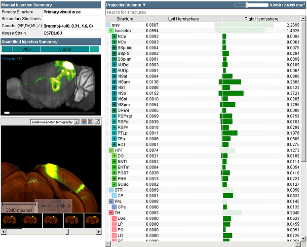
Learn about Image Series Details Mouse Spinal Cord with comprehensive guides and examples from Allen Institute for Brain Science.
Image Series Detail
Gene Symbol
This section shows some gene metadata, including any alternate names for the given gene. If we have data on the same gene in the Allen Brain Atlas project, a link will be included here.If there is a homologue for the current gene in humans and we have data on it in the Human Cortex project of the Allen Institute, a link will be included in this section.
Expression Info

The colored bars in the Expression Info area are a more detailed version of the expression chart from the search result page, as described above. As in the smaller version of the chart, bars are colored green where expression was detected in the corresponding image and white where expression was not detected. There will always be 16 bars in the chart; in cases where an image is not available, the bar will be colored black.
In this detailed view, each bar in the chart is labeled with the image index, tissue index, & annotated segment abbreviation (if available.) The image index refers to the position of the image relative to the image series; these will range from 1 to 16. The tissue index refers to the position of the section relative to the specimen as a whole.
External Resources
The External Resources section contains links to other organizations that provide gene expression data. These links open in a new browser window, and should show information related to the current gene.
Image Detail Page
The image detail page displays the ISH images from one or more image series. A number of different display and formatting options are described below. Use the layout buttons (see below) located on the page toolbar to switch between the various layout options.

Using the Zoom and Pan (Zap) Image Viewer
The default layout shows one or more zoom-and-pan (zap) viewers. The zap viewer allows you to navigate through an image series’ thumbnails to select an image to view at higher resolution. Once selected, you can use your mouse or keyboard to zoom and pan the larger image. Additional image manipulation tools are described below.
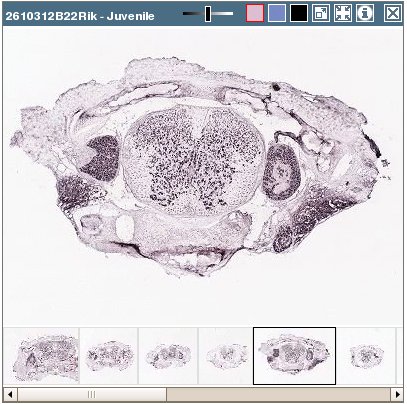
Image Manipulation
Select a thumbnail from the bottom of the image series’ window to open its image in the viewer window. Drag the image with your mouse pointer to an area of interest, then use the plus (+) and minus (-) keys or the wheel on your mouse to zoom in and out.
 | Move the slider bar to the left to intensify the contrast or color. |
|---|---|
   | Select ISH, Nissl or expression mask image type. |
 | Open the selected image in a high-resolution viewer in a new browser window. |
 | Synchronize the images in other viewers on the page to the currently selected image. Only images from specimens of the same age will be synchronized. |
 | Open a new browser window to review metadata for the image series. |
 | Close the viewer. |
Multiple image series can be opened on the same Web page to enable side-by-side comparisons. You can swap viewers’ positions on the page by clicking on the first viewer’s title bar and dragging it to the second viewer’s position.
Alternative Layouts
The layout buttons on the image control toolbar can be used to switch between the contact sheet & row-based views.
The contact sheet layout for a single image series looks like the image to the left. Images are arranged in four rows of four. This view is probably most useful for a single image series.
Multiple image series will be shown in a row-based layout, as shown at right. This view allows all the images from a large number of image series to be visible at one time.
Size

The sizing buttons on the toolbar can be used to change the size of the thumbnails.
By default, the largest thumbnail size is used when viewing a single image series. When multiple series are compared, a smaller thumbnail size will be used. You can override these default values by using the image sizing buttons on the toolbar.

Magnifier

As you move your mouse over each thumbnail, a magnified version of the image will pop up. Use the magnifier buttons to set the size of the magnified image, or disable the magnifier. The currently selected magnifier button will be highlighted with a red border.


To the right are examples of the small & large magnifiers in use.
Clicking on any of the thumbnails will launch a high resolution viewer for that image in a new browser window. See the Single Image Viewer section below for details on working in that view.
Image Type

There are two related images available for each ISH thumbnail:
- The enhanced expression mask. This image is constructed from the signal detected by our image analysis algorithms. This is a grayscale image where the lighter areas indicate stronger signal. Due to the generally low signal, we are showing by default an enhanced version of the expression mask. The bright points in the image have been enlarged and brightened further to make expression more easily discernable in the small thumbnail images presented here. NOTE that clicking on the expression mask thumbnails will open the image in a high resolution image viewer. The expression mask image is not enhanced in the high resolution viewer.
- The closest Nissl stained section. Every tenth section is Nissl stained.
Clicking on the black button in the “associated image” toolbar group (see below)
) will swap out the ISH image and swap in the expression mask image. To return to the ISH image, click on the ISH button (see below).
Button

Clicking on the “nearest Nissl” button (see below) will toggle the display of the nearest Nissl image for each thumbnail. The Nissl image will be displayed beneath its corresponding thumbnail, as shown at left. The nearest Nissl image is available whether the ISH or expression mask thumbnail is currently being shown.
Button
Contrast/Brightness

Use the slider control on the toolbar to increase or decrease the contrast and brightness of the thumbnails. Changing this setting will affect both ISH & expression mask thumbnails, but not Nissl images.
The center position is “neutral,” that is, no enhancement is applied to the images. Moving the slider to the left will darken the images, moving to the right of center will brighten them. To reset the slider to its default position for the type of image currently being displayed, click on the corresponding Image Type button.
The default position for ISH images is “neutral”, while the default position for expression mask images is about +80% brightness.
Learn about Search Mouse Spinal Cord with comprehensive guides and examples from Allen Institute for Brain Science.
Searching
There are two ways to search the data on the "Spinal Cord " site; “Gene Search” and “Advanced Search.”
Gene Search
“Gene Search” appears on our landing page. A gene search will show you a list of all the experiments we’ve done involving a gene that matches your search criteria. A “Match” in gene search means that the text you type in is contained somewhere in the name, symbol or alternate symbol of the gene involved in the experiment.
As you begin typing in the gene search box, a list of suggestions will appear. You can use your arrow keys or the mouse to move down, highlighting the desired entry. If you’re using your mouse, click on the desired entry to select it, then hit your “Enter” key or click the Search button to perform the search. If you’re using arrow keys, hit the “Enter” or “Tab” key to select the highlighted item. If you don’t want to use any of the suggestions, hit your “Esc” key or click your mouse outside the list and it will disappear.
Advanced Search
The Advanced Search page has many more options. You can:
- Use the check boxes to limit a gene search to any combination of gene name, symbol or alternate symbols.
- Search by EntrezGene ID, or by our internal Image Series ID.
- Search by specimen age.
Type-ahead suggestions will appear for the gene search and all of the ID entry fields. After selecting a suggestion, click the Search button or hit the Enter key to perform your search. As noted above, you can dismiss the list of suggestions by hitting the “Esc” key.
Search Results
The result set shows a collection of gene expression experiments.
Please note-- If you searched by gene, it may appear that some of the rows do not match your gene criteria. Keep in mind that by default all of the alternate gene symbols (which are not shown in the result list) are included in a gene search. To see the alternate symbols for a gene, click on the gene symbol in the result list. If you want to exclude alternate symbols from your gene search, try the Advanced Search page.
Expression charts
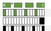
Each of our experiments is divided into 16 images, covering the length of the spinal cord. Each row in the result set contains a small expression chart that describes in which images expression was detected for the given gene. As shown in the example at left, each chart is divided into 16 bars, one for each image in the image series. If expression was detected in an image, its corresponding bar will be colored green. If no expression was detected, the bar will be colored white. If a section image is unavailable, its position will be colored black. The sections progress from rostral to caudal, reading left to right.
Expression Categories
This chart appears on the search results page and is meant to indicate membership in the various “expression enrichment” categories for each experiment.
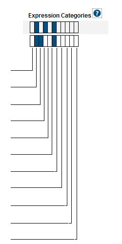
A dark blue rectangle indicates membership in the corresponding category. The category positions are described below; you can also hover your mouse over a blue rectangle to show the category name.
- Laminae 1-3
- Laminae 4-6
- Laminae 7-8
- Laminae 9
- Intermediolateral Column
- Gray Matter
- White Matter
- Central Canal
- Ventral-dorsal Midline in Gray Matter
- Radially Arrayed in White Matter
- Vascular-like in Gray and White Matter
Sorting
The results are initially sorted by Gene Symbol in ascending order. Click on any of the column headers to sort by that column; click on the same column header again to reverse the sort order. A small arrow will appear next to the currently sorted column, indicating the sort order, as shown in the image at right.It is also possible to sort by expression position. In the expression chart illustration above, note the rectangular green blocks in the top row. Clicking one of these boxes will sort the results according to amount of expression in the corresponding area of the specimen. Each of the sort-boxes represents an area covering four images in the specimen. The first box (labeled “R” for Rostral) represents the four most-rostral images; the last box (labeled “C” for caudal) represents the four most-caudal images, and so on.
Getting more detailed information
The Gene Symbol links to detailed information about the gene in our experiments. The number in the “Images” column links directly to a contact sheet of all the images for the given experiment.
Comparing Result Sets

In addition to the links found in each experiment row, you can select multiple rows to compare side-by-side. Click the check box at the far left of the desired rows, then click the “Compare Selected Experiments” button. Use the check box in the column header to toggle all of the row check boxes on or off.
XML
As shown in the image above, at the bottom of the table there is a link to an XML document containing all of the data in the result set.
Learn about Allen Brain Explorer Beta User Guide with comprehensive guides and examples from Allen Institute for Brain Science.
The Allen Brain Explorer (beta) is a browser-based 3D visualization tool to explore multimodal data in an integrated, anatomically annotated, spatial framework. This initial release allows users to explore the Allen Mouse Brain Connectivity Atlas projection data and Allen Reference Atlas (ARA) in a standardized coordinate space. Future releases will add functionality and additional data. Users are encouraged to provide bug reports or other feedback via Send Us A Message.

Browser Compatibility
The following web browsers have been tested for support, using updated versions as of June 2018:
- Edge (HTML 16, Windows 10 Fall 2017 Creator’s Update)
- Firefox 59
- Chrome 66
- Safari 11.1
Browser Navigation Controls
At this time, this application supports use of a clickable mouse for selecting and interacting with data.
View Brain Anatomy
The Allen Brain Explorer displays anatomical structures defined in the Allen Mouse Common Coordinate Framework (CCF). Briefly, this space is created using a population average of 1,675 C57/Bl6 adult mouse brains, with 662 annotated structures rendered in 3D. Refer to the CCF technical whitepaper for more details on creation and annotation of this reference atlas and spatial framework.

Navigation Tools: Anatomical Annotated Reference Planes and Grid
Open coronal, sagittal, and horizontal slice planes by clicking the Toggle Reference Planes button. Each plane displays the structural boundaries of the annotated brain areas. Drag the colored arrows to move the slice planes. A grid can be toggled to provide approximate spatial scale. Future releases will include accurate scale information.
Anatomical Structure Ontology
Access and visualize brain structures by interacting with the Anatomical Ontology list. This box provides a searchable hierarchical organization of brain structures.
- Click on the white arrowhead next to a structure to view its sub-structures.
- Display or hide the 3D representation of a particular structure by clicking the “eye” icon next to the structure.
- Search for structures by typing the name or abbreviation in the text box next to the magnifying glass icon.
- View anatomical structures with opaque or semi-transparent color schemes using the toggle slider in the header of this box. The default setting is opaque.
View Axonal Projections
The Allen Mouse Brain Connectivity Atlas contains icons to access data via this Allen Brain Explorer viewer. Users can visualize anatomically mapped projection pathways, and explore more detailed experimental information, including image data. The Allen Brain Explorer can be accessed from three other sources throughout the Allen Mouse Brain Connectivity Atlas, using the icons highlighted in red below:

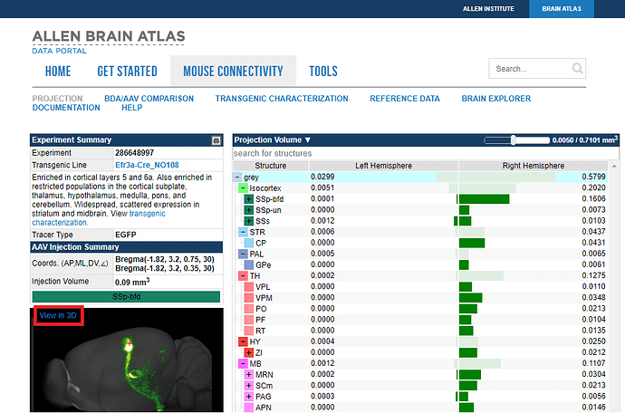
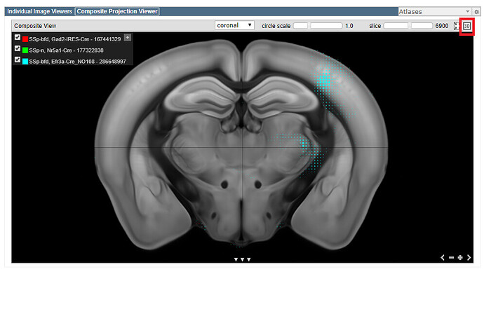
When one or more projection data sets are selected, they will be loaded into the Allen Brain Explorer, and displayed in the Virtual Tractography box. Primary data images can then be viewed by clicking either on injection site or projection site voxels and launching via the Source Image tab in the Experiment Information box. More data sets can be added to the Allen Brain Explorer view either by continuing to select data using the access described above, or by directly typing Experiment IDs into Virtual Tractography box.
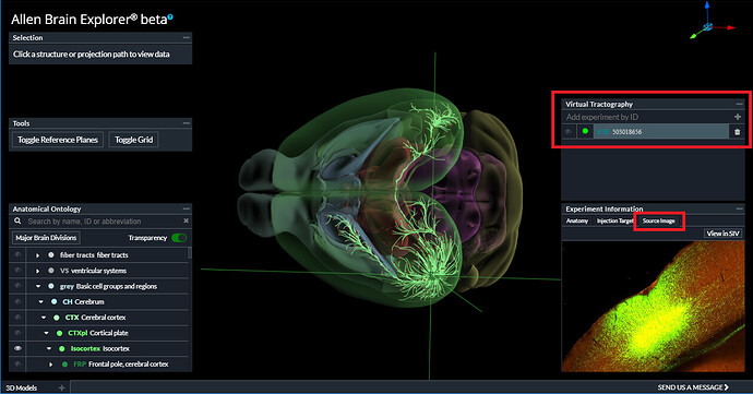
Problems? Suggestions? Users are encouraged to provide bug reports or other feedback via Send Us A Message, located in the lower right of the Allen Brain Explorer, or in the footer of other pages of the Allen Brain Atlas portal. Include reference to the Allen Brain Explorer in your message.
Learn about Expression Mask Color Maps with comprehensive guides and examples from Allen Institute for Brain Science.
Visualization/Analysis Tool

The expression mask images you see on this site start out as gray scale images, with low expression appearing as black, and increasingly high expression showing as increasingly bright white. By default, we apply a color map to make the difference between high and low expression more distinct. On the color map page , you can choose how colors are mapped to expression masks. Your choice is stored in a javascript cookie on your computer. This means that your choice will stay in effect until either you return to the color map page to change it, or the cookie is deleted from your computer. It also means that your web browser must be configured to accept cookies, which is already the case for the great majority of users
Click here to go to the expression mask color map page.
Learn about Transgenic Mouse Lines Allen Brain Observatory with comprehensive guides and examples from Allen Institute for Brain Science.
Transgenic Strategy
The Allen Brain Observatory contains data collected via two-photon calcium imaging to quantify neuron activity in the mouse neocortex in response to visual stimuli. The use of a fluorescent calcium indicator, GCaMP6f, was used to image neural activity in the visual cortex of transgenic mice exposed to various visual stimuli. Calcium influx associated with neural activity results in transient increases in fluorescence of GCaMP6-GFP. These experiments use the transgenic mouse line Ai93, in which GCaMP6f expression is dependent on the activity of both Cre recombinase and the tetracycline-controlled transactivator protein (tTA). Triple transgenic mice (Ai93, tTA, Cre) were generated by first crossing Ai93 mice with Camk2a-tTA mice, which preferentially express tTA in forebrain excitatory neurons. Double transgenic mice were then crossed with a Cre driver line to generate mice in which GCaMP6f expression is induced in the specific populations of neurons that express both Cre and tTA.
Transgenic Mouse Lines
Specific expression is driven by the following Cre driver lines. Clicking on one of the links below will open serial two-photon images of fluorescent GCaMP6-GFP expression in the triple transgenic mouse line in an image viewer.
In the Transgenic Characterization section of the Allen Brain Observatory, each of the above cell lines is listed with links to view the 2-photon serial tomography as well as a brief description of the brain areas targeted by the transgenic strategy. To view the fluorescence expression in these mouse lines in an image viewer, click on either the transgenic mouse line or the example image.
Viewing Fluorescence Images
Transgenic Mouse Detail Page
Clicking on either the transgenic mouse line name or the example image will open a transgenic mouse detail page with metadata on the mouse line including the line name, age, plane of sectioning, organism, sex and induction method.

A panel of images also shows each section (~140 sections) from this series of images. Scrolling down the page will allow you to see images with fluorescence expression. Clicking on one of the individual images will open a high resolution image viewer in a new tab.

Image Viewer

The Image Viewer is a powerful tool to navigate and view the images in this series. The main viewer contains a scale bar, a toolbar and on-screen navigation tools. The main viewer is an interactive window where an image can be repositioned by clicking on the image and dragging with the mouse. Use the scroll wheel, on-screen navigation buttons or the keyboard to zoom in or out. The name of the mouse line and the expressed fluorescent molecule is displayed in the top left-hand corner of the main viewer.
Thumbnails for the entire image series are displayed across the bottom of the main viewer in section order. Click a thumbnail to select that image for viewing, or use the keyboard to navigate through the series.
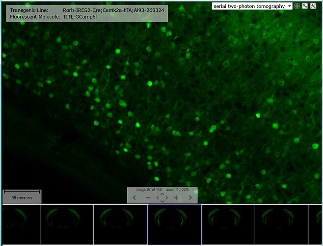
Scale Bar
Drag the scale bar with your mouse to the desired location. Click the scale bar text with your mouse to toggle between horizontal and vertical scale bars.
Using the Image Viewer Toolbar
Use the toolbar to take actions on the current image. Toolbar controls include:
| Icon | Function |
|---|---|
 | Clicking the key icon will open another viewer with the reference atlas |
 | Once the reference atlas is open, this icon, when clicked, will sync the other viewer to the same location |
 | Opens the tools menu |
 | From the reference atlas menu, allows for the atlas images or the nissl images to be displayed |
From the reference atlas menu, allows for the atlas images or the nissl images to be displayed
Keyboard Commands
Use the keyboard to navigate through the image series and synchronize the viewers on the page. Keyboard commands include:
Tools Menu
The tools menu allows access to downloading both the fluorescence and reference atlas images, as well as to remove the metadata information on the atlas and fluorescence images (to allow for a cleaner screen-shot).
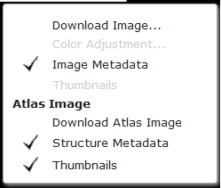
Learn about Data Visual Coding with comprehensive guides and examples from Allen Institute for Brain Science.
Neuronal Response: Two-Photon Calcium Imaging
The first data modality to be released from the Allen Brain Observatory is a standardized in vivo survey of physiological activity in the mouse visual cortex, featuring representations of visually evoked calcium responses from GCaMP6-expressing neurons at selected cortical depths and visual areas.
Experiment Design
In this study, an experiment is composed of three one-hour long two-photon calcium imaging sessions on an awake mouse presented with a series of visual stimuli. An experiment is the unique combination of one mouse, one imaging depth (e.g. 175 um from surface of cortex), and one visual area (e.g. “Anterolateral visual area” or “VISal”). Each experiment includes three imaging sessions as illustrated below. Data released in the June 2016 and October 2016 releases were collected using sessions A, B and C. Data released in the June 2017 release were collected using sessions A, B and C2.
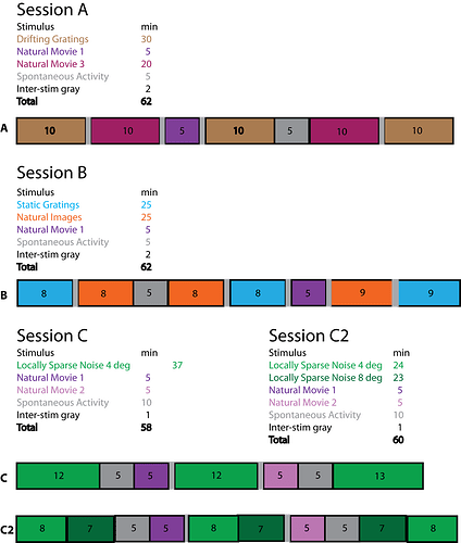
For more information on the experimental design and the visual stimulus set, see the Stimulus Set and Response Analysis whitepaper in Documentation.
Targeted Functional Visual Areas
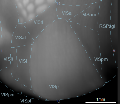
*Wang and Burkhalter (J.Comp.Neurol., 502: 339-357. doi: 10.1002/cne.21286)
Transgenic Lines
Two-photon calcium imaging was recorded in neurons expressing a calcium-sensitive fluorescent molecule. This is made possible by the use of animals harboring a genetically encoded calcium sensor, GCaMP6, which is imparted by use of the Ai93 line and expressed in subsets of cell populations due to a combinatorial transgenic line breeding strategy. The transgenic lines are a cross of CaMK2a-tTA - a transgene directing tetracycline-controlled transactivator protein (tTA) expression in forebrain excitatory neurons - and one of the following:
- Cux2-CreERT2
- Rorb-IRES2-Cre
- Rbp4-Cre_KL100
- Nr5a1-Cre
- Scnn1a-Tg3-Cre
- Emx1-IRES-Cre
Histological characterization for each of these triple transgenic mouse lines is available by clicking on the Transgenic Characterization tab in the menu banner. Further characterization of each of these transgenic lines can be found in the Transgenic Mouse Catalog in Documentation.
Searching the Data
The data can be searched either by experiment or by cellular response. To search for experiments or cells that have specific response characteristics, click on the respective Experiments tab or Cells tab from the menu banner.

Exploring the Data from the Interactive Landing Page
The Allen Brain Observatory includes a variety of data visualization summaries capturing visual coding properties of single cell and cell population responses to visual stimuli. This resource introduces new visualizations that summarize the cellular responses for each visual stimulus in a single figure:

The Visual Stimulus pages include details on how to interpret these visualizations and how they were created. Clicking the stimulus from the panel below the cortical imaging locations to reach these pages.

The landing page shows a visual summary of the dataset contents. Transgenic mouse lines (left panel) were selected based on the subpopulation of neurons expressing GCamp6. From the landing page, you can explore the transgenic mouse line, cortical area and cortical depth of the experiments conducted in this study. Hovering your mouse over the transgenic lines, cortical area or cortical depth will highlight the parameters captured in the experiments of this study. Clicking one of these interactive links will return a Cell Search with those specific criteria.
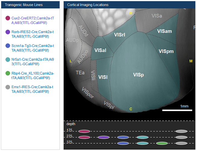
Below the visual stimulus links are another interactive search feature that will return a list of cells that responded to the visual stimulus. Click one of the links to perform this kind of search.

Experiment Search


Clicking “Experiments” in the menu banner will take you to a Experiment Search page. By default, all experiments conducted in this study are listed on this page. The list of experiments can be sorted/filtered by clicking the “Show Filters” button which opens options for selecting experiments by Brain Area (VISal, VISp, VISl, VISpm, VISam, VISrl), Imaging Depth in microns (175, 265, 275, 300, 320, 335, 350, 365, 375, 435) or by Cre Driver (Rbp4-Cre_KL100, Cux2-CreERT2, Emx1-IRES-Cre, Scnn1a-Tg3-Cre, Rorb-IRES2-Cre, Nr5a1-Cre).
Each experiment is displayed by a row in the results list below the Filters menu. All of the columns (minus the two common mouse lines) are displayed by default. Columns can be hidden by deselecting them from the drop-down menu. The population thumbnails are segregated by visual stimulus as indicated by the stimulus color key. Overall cell population responses of the neurons in the imaging field of view to a specific visual stimuli are displayed as population thumbnails and can be explored in more detail from the Experiment Detail Page. More information on how these features were computed can be found in the Stimulus Set and Response Analysis whitepaper located in Documentation.
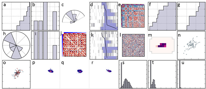
Experiment Detail Page
Each experiment is composed of three approximately one-hour two-photon calcium imaging sessions.The experiment detail page presents a more detailed view of each experiment including detailed experiment information, summary images of the cortical field of view in each experiment and the calculated cell population features and metrics as represented by the population thumbnails.
Detailed information about each experiment is listed at the top of the page, including mouse genotype information, cortical area imaging depth that the data was acquired from, a link to the Cell List - which summarizes the cell responses for each of the two-photon calcium imaging sessions, and experimental series identifier. Some experiments will have notes with information about special considerations, such as animal physiology. Summary images of the cortical field of view from each of the imaging sessions are also shown.

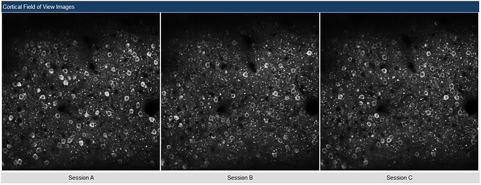
Population Thumbnails
The cortical field of view that is captured in a single imaging session is referred to as the “population” of cells that are recorded simultaneously. Population image thumbnails are shown on the Experiment Search page, with a description of the data that may be available from each of these sessions.
Cell Search
Clicking the “Cells” tab from the menu banner will open a search page from which all the cells from every experiment can be filtered and sorted. Filtering subselects cells that meeting the filtering criteria, while sorting orders the cells (filtered or not) by the selected metric. Clicking the interactive panelsfrom the Allen Brain Observatory landing page or the “View Cells” link from an Experiment Detail Page will open the Cell Search page with filtering already pre-set.
Cell List
This page displays the cellular response summaries of a cell search with one cell per row. Clicking anywhere on a row will take you to the Cell Detail Page. More information on the development of each of the thumbnails and it’s corresponding visual stimulus can be found from the “Visual Stimuli” buttons on the Overview page.

Filtering Cells
To filter the cells based on cellular responses across all the experiments, first click on the “Show filters” button at the top left-hand corner of the webpage.
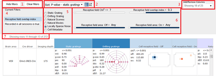
- Filters: Show, hide or clear filters by clicking these buttons
- Sort: Sort by parameter and choose either ascending or descending sort
- Add/Remove Columns: Increase or decrease the number of columns shown in your cell search results
- Current Filters: Filters will show in the box once applied
- Filter Parameters: Clicking a radio box will determine which visual stimulus or metadata parameters you can filter on
- Filter Criteria: Parameters are visual stimulus and metadata dependent.
- Row Number: The number of cells included in the filter criteria
More information can be found on these thumbnails and metrics from the Cell Detail Page
Sorting Cells
By default the cells are sorted based on the significance of their measured responses to presentation of the static grating, listed here as their p-value, but can also be sorted by several other parameters from the “Sort” drop-down menu. The list of cells includes metadata on the experiment (Brain area, Cre driver, Imaging depth) and 23 response summaries (including visualizations and computed metrics) to the various visual stimuli. Of the 23 columns available, only 18 are displayed by default, but can be displayed from the “Add/Remove Columns” drop down menu in the filters box. Sorting is based on the calculated features derived from the cellular responses to the visual stimuli.

Cell Detail Page
Information at the level of the individual cell is available from this page. Similar to the Experiment Detail Page the top of the page provides detailed information from the experiment from which this cell was imaged.

For every stimulus that the selected cell was responsive to, a large thumbnail will be available to interact with. Hovering your mouse over the thumbnail will reveal the the selected visual stimulus. Each thumbnail also includes metrics calculated from the cell responses. clicking the “i” next to a visual stimulus will link to the webpage explaining both the stimulus as well as the thumbnail plot developed to describe the cellular response. Clicking on the stimulus in the table below will link to those same pages.
Learn about Microarray Data For NHP Atlas with comprehensive guides and examples from Allen Institute for Brain Science.
There are two sets of microarray data in this resource; Micro- and macrodissection studies, both assayed on the Affymetrix GeneChip Rhesus Macaque Genome Arrays. The Macrodissection study includes microarray data assayed from samples that were dissected manually from four postnatal stages in five specific sample tissue locations; medial frontal cortex (areas 24, 25 and 32), occipital cortex, hippocampal cortex (hippocampal formation), amygdaloid complex and basal nuclei (basal ganglia). The Microdissection study looks at smaller more targeted subdivisions of the structures considered in the macro study in four postnatal stages and six prenatal stages. These smaller regions, such as a single cortical layer of cells, were microdissected using a laser dissection microscope. To choose between these data sets, select “Microdissection” or “Macrodissection” from the Microarray drop down menu.
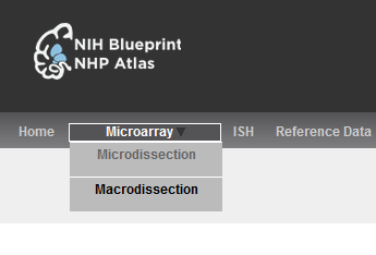
Microdissection Microarray
Searching
You can browse the data using the three search tools: (1) Gene Search, to obtain gene expression data for specific genes of interest, (2) Differential Search, to compare expression between two sets of brain structures at desired developmental stages, and (3) Correlative Search, to find genes that have an expression pattern similar to a “seed gene” selected from the results of a Gene or a Differential search.
Some search modes offer additional information, accessible by clicking on the “?” next to the Search button.
Gene Search
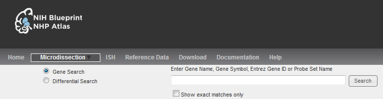
To search for probes associated with a specific gene, select the Gene Search radio button, type the gene name, gene symbol or Entrez Gene ID in the search box and click the “Search” button. You can also select an entry from the list displayed as soon as you start typing. To be able to search the Macaque database for human gene homologues, search using:
- gene symbol
- gene aliases
- gene name
- Entrez ID (NCBI)
- Ensembl ID
- Affymetrix Probeset ID
The search results are displayed in the form of a heat map showing the expression values for the probes that match the search criteria. Since the microarray may have more than one probe per gene, the heat map’s left panel shows Gene Symbol and Probe Name for each row.
Gene symbols and gene names are displayed as follows:
- If the probe targets a Macaque NCBI gene then the gene abbreviation will be displayed unaltered (eg. CLEC1A)
- If the probe targets a Human NCBI gene then the gene abbreviation will be displayed inside parentheses (eg. (CLEC1A))
- If the probe targets a Macque Ensembl gene then the gene abbreviation will be appended with the Ensembl ID in parentheses (eg. CLEC7A(ENSMMUG00000002192))
- If the probe targets a Macque Ensembl gene and there is no available gene name, then the Ensembl ID will be used as the gene name (eg. ENSMMUG00000018691)
See Microarray Data Visualization for information on reading heat maps.
Differential Search
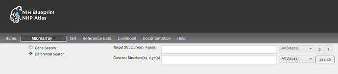
This dataset can be searched to find genes that show enrichment of expression in one set of samples compared to another set of samples. Those samples can correspond to different brain structures and/or different developmental stages. To perform this type of query, select the “Differential Search” radio button. To find genes or probes with enhanced expression profiles in a target set of samples when compared to a contrast set of samples, first select the Target and Contrast Structures by starting to type the structure name in the text box - a structure ontology of the applicable structures will appear and you can select from this menu. Then, select the desired developmental stages using the Ages drop down boxes for both the Target and Contrast Domains.
You can reverse Target and Contrast Domains by pressing the toggle button above the Search button.
Search Results

The search results will shown in the form of a Heatmap with genes that exhibit higher expression in the target domain ranked higher than those in the contrast domain by either p-value or by fold change. To alter the sort parameter, click on either the “p-value” or the “Fold Change” buttons. Since the macaque genome is not fully annotated, many probes do not have a corresponding associated gene. In those cases, the probe name is displayed under the Gene Symbol label.
Correlative Search
Since genes with similar expression patterns may be related in function, the NHP Atlas includes functionality to search the dataset for genes whose expression over a given set of structures or developmental stages resemble the expression pattern of a gene of interest.

First, the gene of interest must be selected from the heatmap returned by a Gene or Differential search by clicking on a data-point in the heatmap. The corresponding probe will be displayed under the “Find Correlates” button close to the top right corner of the heatmap. Next, select the desired structures and developmental stages from the drop down menus and then click “Find Correlates”.
The resulting heatmap displays the list of probes based on the search criteria ranked by Pearson’s correlation “r” with the gene of interest. To find the anti-correlate, click the “r” button.
To filter the heatmap display to show specific structures or developmental stages, use the “Filter Heatmap” function at the bottom of the heat map.
Microarray Data Visualization
The results for all three types of searches against microarray data are displayed in two horizontal page sections:
- The bottom section contains the heat map representation of the data returned by the search operation.
- The top section contains probe, sample and expression information for the data point selected by clicking on a cell in the heat map.
Heatmap
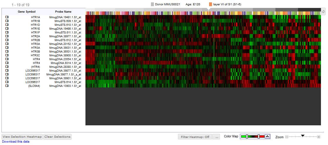
Based on your search, the resulting microarray data are presented as a matrix with brain structure and developmental stage on the horizontal x-axis and gene probes on the vertical y-axis. On the horizontal axis, developmental stages are represented on top, color coded in shades of gray such that moving from left to right corresponds to increasing age. Brain structures are represented in bright colors immediately below, such that moving left to right corresponds to moving in the anterior to posterior direction, first in the cortical areas, followed by subcortical areas, cerebellum and brainstem.
Each column therefore represents a structure for a specific developmental stage. On the vertical axis, each row represents a probe rather than a gene, because multiple probes were used to measure gene expression for a gene. Additionally, since the macaque genome is not fully annotated, many probes do not have a corresponding associated gene. In those cases, the probe name is displayed under the Gene Symbol label.
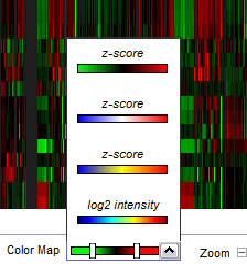
The microarray data is presented in a heat map format where the colors of the heat map correspond either to normalized data (log2 Intensity) or to a normalized (z-score) expression level of a probe. Default heat map colors the z-score in the green – red scale, where green represents underexpression and red overexpression of that gene compared to expression throughout the brain. The window and level for the colors may be adjusted, and other color schemes may be selected, by using the Color Map control under the heat map. The slider on the bottom right can be used to adjust the zoom level. In the top right hand corner of the heat map, there is a toggle button, which when clicked will sort the heat map data either by donor or by structure.
To view expression patterns of the returned probes in specific regions of the brain or in specific developmental stages, filter the heatmap display from the function below the heat map.
You can select a set of probes for later use by checking the checkboxes besides the list of gene symbols. Your choices are stored in a browser ‘cookie’ in your computer and will remain in effect until you click the “Clear Selections” button or clear your web browser’s cookie cache. Click the “View Selection Heatmap” button to see your selections.

Clicking on a heat map cell populates the top section of the page with detailed information about that cell. This information includes gene symbol, gene name, NCBI Entrez ID, probe name, chromosome, as well as the sample’s structure and specimen’s age. It also shows the exact expression values by their log2 intensity and z-score.
The section also contains buttons to navigate to related data in other Allen Brain Atlas resources.
Filter Heatmap
If you are interested in narrowing the number of donors or structures, use the “Filter Heatmap” function below the heatmap. Clicking on the “…” button will bring up a menu where you can choose the donors and structures you’d like to visualize. Once you have saved your options, turn on the Filter Heatmap function by clicking the button.
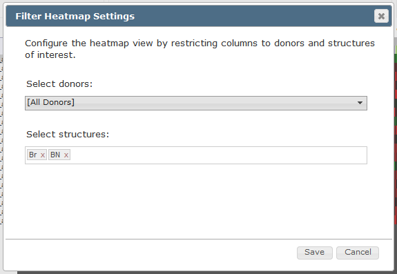
Macrodissection Microarary
This dataset includes microarray data manually dissected from five brain regions; medial frontal cortex (areas 24, 25 and 32), occipital cortex, hippocampal cortex (hippocampal formation), amygdaloid complex and the basal nuclei (basal ganglia), from four post-natal stages.
Searching
You can browse the data using the three search tools: (1) Gene Search, to obtain gene expression data for specific genes of interest, (2) Differential Search, to compare expression between two sets of brain structures at desired developmental stages, and (3) Correlative Search, to find genes that have an expression pattern similar to a “seed gene” selected from the results of a Gene or a Differential search.
Some search modes offer additional information, accessible by clicking on the “?” next to the Search button.
Gene Search
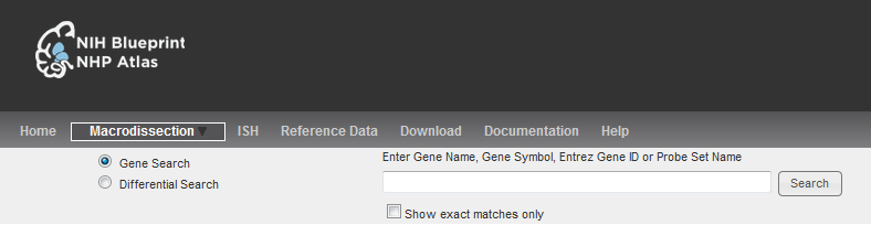
To search for probes associated with a specific gene, select the Gene Search radio button, type the gene name, gene symbol or Entrez Gene ID in the search box and click the “Search” button. You can also select an entry from the list displayed as soon as you start typing. To be able to search the Macaque database for human gene homologues, search using:
- gene symbol
- gene aliases
- gene name
- Entrez ID (NCBI)
- Ensembl ID
- Affymetrix Probeset ID
The search results are displayed in the form of a heat map showing the expression values for the probes that match the search criteria. Since the microarray may have more than one probe per gene, the heat map’s left panel shows Gene Symbol and Probe Name for each row.
Gene symbols and gene names are displayed as follows:
- If the probe targets a Macaque NCBI gene then the gene abbreviation will be displayed unaltered (eg. CLEC1A)
- If the probe targets a Human NCBI gene then the gene abbreviation will be displayed inside parentheses (eg. (CLEC1A))
- If the probe targets a Macque Ensembl gene then the gene abbreviation will be appended with the Ensembl ID in parentheses (eg. CLEC7A(ENSMMUG00000002192))
- If the probe targets a Macque Ensembl gene and there is no available gene name, then the Ensembl ID will be used as the gene name (eg. ENSMMUG00000018691)
See Microarray Data Visualization for information on reading heat maps.
Differential Search
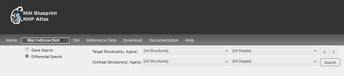
This dataset can be searched to find genes that show enrichment of expression in one set of samples compared to another set of samples. Those samples can correspond to different brain structures and/or different developmental stages. To perform this type of query, select the “Differential Search” radio button. To find genes or probes with enhanced expression profiles in a target set of samples when compared to a contrast set of samples, first select the Target and Contrast Structures from the drop-down menu. Then, select the desired developmental stages using the Ages drop-down boxes for both the Target and Contrast Domains.
You can reverse Target and Contrast Domains by pressing the toggle button above the Search button.
Search Results
The search results will shown in the form of a Heatmap with genes that exhibit higher expression in the target domain ranked higher than those in the contrast domain by either p-value or by fold change. To alter the sort parameter, click on either the “p-value” or the “Fold Change” buttons. Since the macaque genome is not fully annotated, many probes do not have a corresponding associated gene. In those cases, the probe name is displayed under the Gene Symbol label.
Correlative Search
Since genes with similar expression patterns may be related in function, the NHP Atlas includes functionality to search the dataset for genes whose expression over a given set of structures or developmental stages resemble the expression pattern of a gene of interest.
First, the gene of interest must be selected from the heatmap returned by a Gene or Differential search by clicking on a data-point in the heatmap. The corresponding probe will be displayed under the “Find Correlates” button close to the top right corner of the heatmap. Next, select the desired structures and developmental stages from the drop down menus and then click “Find Correlates”.
The resulting heatmap displays the list of probes based on the search criteria ranked by Pearson’s correlation “r” with the gene of interest. To find the anti-correlate, click the “r” button.
To filter the heatmap display to show specific structures or developmental stages, use the “Filter Heatmap” function at the bottom of the heat map.
Microarray Data Visualization
The results for all three types of searches against microarray data are displayed in two horizontal page sections:
- The bottom section contains the heat map representation of the data returned by the search operation.
- The top section contains probe, sample and expression information for the data point selected by clicking on a cell in the heat map.
Heatmap
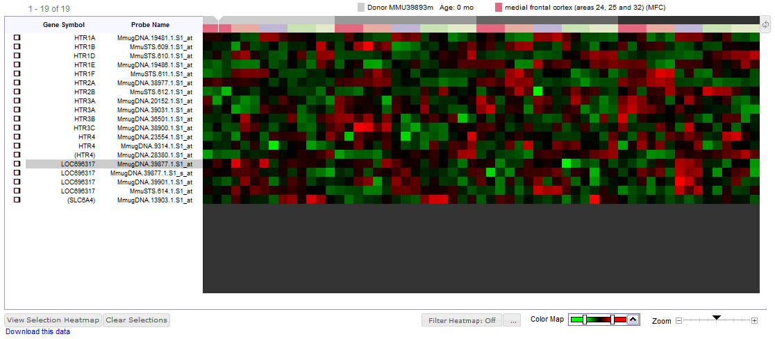
Based on your search, the resulting microarray data are presented as a matrix with brain structure and developmental stage on the horizontal x-axis and gene probes on the vertical y-axis. On the horizontal axis, developmental stages are represented on top, color coded in shades of gray such that moving from left to right corresponds to increasing age. Brain structures are represented in bright colors immediately below, such that moving left to right corresponds to moving in the anterior to posterior direction, first in the cortical areas, followed by subcortical areas, cerebellum and brainstem.
Each column therefore represents a structure for a specific developmental stage. On the vertical axis, each row represents a probe rather than a gene, because multiple probes were used to measure gene expression for a gene. Additionally, since the macaque genome is not fully annotated, many probes do not have a corresponding associated gene. In those cases, the probe name is displayed under the Gene Symbol label.
The microarray data is presented in a heat map format where the colors of the heat map correspond either to normalized data (log2 Intensity) or to a normalized (z-score) expression level of a probe. Default heat map colors the z-score in the green – red scale, where green represents underexpression and red overexpression of that gene compared to expression throughout the brain. The window and level for the colors may be adjusted, and other color schemes may be selected, by using the Color Map control under the heat map. The slider on the bottom right can be used to adjust the zoom level. In the top right hand corner of the heat map, there is a toggle button, which when clicked will sort the heat map data either by donor or by structure.
To view expression patterns of the returned probes in specific regions of the brain or in specific developmental stages, filter the heatmap display from the function below the heat map.
You can select a set of probes for later use by checking the checkboxes besides the list of gene symbols. Your choices are stored in a browser ‘cookie’ in your computer and will remain in effect until you click the “Clear Selections” button or clear your web browser’s cookie cache. Click the “View Selection Heatmap” button to see your selections.
Clicking on a heat map cell populates the top section of the page with detailed information about that cell. This information includes gene symbol, gene name, NCBI Entrez ID, probe name, chromosome, as well as the sample’s structure and specimen’s age. It also shows the exact expression values by their log2 intensity and z-score.
The section also contains buttons to navigate to related data in other Allen Brain Atlas resources.
Filter Heatmap
If you are interested in narrowing the number of donors or structures, use the “Filter Heatmap” function below the heatmap. Clicking on the “…” button will bring up a menu where you can choose the donors and structures you’d like to visualize. Once you have saved your options, turn on the Filter Heatmap function by clicking the button.
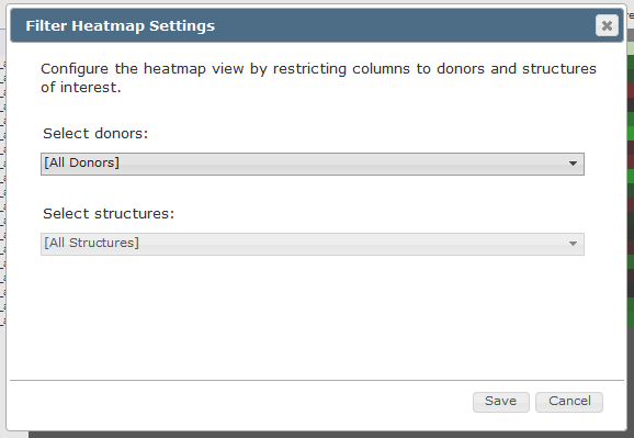
Learn about High Resolution Image Viewer with comprehensive guides and examples from Allen Institute for Brain Science.
Launching Viewer

Click on any thumbnail image in this application to launch the high resolution viewer in a new browser window. This viewer provides an efficient way of viewing very large, high resolution images over relatively low bandwidth.
Zoom/Pan

Use the controls shown at left to zoom and pan around the image. You can also zoom by clicking on the image, and pan by click-and-dragging the image, or using the keyboard up/down/right/left arrow keys.
Tool Box
The tool box shown at right enables you to
- Switch between an ISH image and its corresponding expression mask or closest Nissl image.
- Page through all the images in the same image series.
- Adjust contrast & brightness (on the “Properties” page.)
- Email a link to the image (Tools page.)
- Download a JPEG of the image (Tools page.)
Note: all downloaded images will have rotation of 0 degrees

Scaling
The scale key will change appropriately as you zoom in and out of the image. Click and drag the key to any position on the image to measure regions of interest. Click on the text to flip the scale from horizontal to vertical.
The position key shows approximately where the current section comes from, relative to the specimen as a whole.
Rotate Control
The rotate control allows you to rotate the image to manipulate viewing orientation. Please note that if you download a JPEG of the image (see tool box description above), the image will not have any rotation applied to it; it will have a rotation of 0 degrees.
Learn about Overview Allen Brain Observatory with comprehensive guides and examples from Allen Institute for Brain Science.
Rationale and Experimental Overview
The Allen Brain Observatory provides a rich dataset for investigating how visual stimuli are represented by neural activity in the mouse visual cortex in both single cells and populations. A standardized data acquisition pipeline was established, utilizing two-photon calcium imaging as a means of recording visually evoked responses from animals performing a visual perception task. Primary and secondary areas of the visual cortex in different transgenic mouse lines harboring G-protein coupled calcium-responsive reporters (GCaMP6) in selected cell subpopulations were analyzed during exposure to five classical visual stimuli, providing a growing dataset to survey information encoding in the visual cortex.
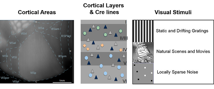
Defining visually responsive areas of the cortex
Intrinsic signal imaging (ISI) measures hemodynamic response to sensory stimulation across a wide field of view and thus was used to achieve a “retinotopic map” to represent the spatial relationship of stimuli in the visual field to corresponding locations within responsive cortical areas. Retinotopic mapping was used to establish the anatomical boundaries of functionally defined visual areas, and was used to target in vivo two-photon calcium imaging to selected locations in primary and secondary visual cortical areas.
For more information on how ISI was performed and analyzed, refer to the Overview whitepaper in Documentation.
Visual Stimulus and Neuronal Response
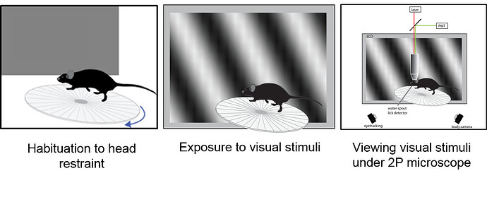
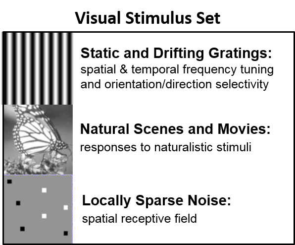
Neuronal activity was measured in GCaMP6-expressing neurons from selected populations defined by depth and Cre line. For more information on the characteristics of these transgenic lines, see the Transgenic Line Catalog in Documentation.
Video recordings of the visual cortex were gathered during presentation of the various visual stimuli. Activity of the neurons in response to stimuli was detected as transient increases in cellular fluorescence on a millisecond time scale. The data processing of these raw movies involved motion correction and image segmentation to identify the sets of pixels representing distinct cells, and activity of these identified neurons was extracted as traces for quantification. Ultimately, the activity of each responsive cell may be correlated to the visual stimulus that was viewed by the mouse.
Availability of 2-photon calcium fluorescence movies
Motion-corrected 2-photon calcium fluorescence movies are too large to download conventionally, but are available upon request. Each experiment contains three movie files of approximately 60 GB each. We ask that anyone requesting movies provide one or more hard drives with sufficient capacity to store the files and a shipping number from your organization for return. These will be returned after file transfer is complete. Data is provided under the Allen Institute Terms of Use policy.
To request movie files, please contact us to indicate:
- desired movies from specific experiments
- point of contact name and email address
- organization
- area of research
- proposed use of the data
Upon receipt of this message, arrangements will be made with the point of contact and will usually be complete within two weeks of the receipt of a storage drive.

Exploring the data
To learn more about the visual stimulus set as well as the data visualizations that were created to represent the cellular responses, see the visual stimulus pages:
To view characterization of the transgenic mouse lines used in this study, see the Transgenic Characterization tab.
To view the data by experiment click on the Experiments tab.
To search the experiments for cells with certain response criteria, click the Cells tab.
To download the data, visit the Download page.

Learn about Documentation Mouse Spinal Cord with comprehensive guides and examples from Allen Institute for Brain Science.
Available Files
Learn about In Situ Hybridization ISH Data For NHP Atlas with comprehensive guides and examples from Allen Institute for Brain Science.
Searching
This study collected high-resolution in situ hybridization image data covering selected genes during development. For a list of genes, please see the gene list under the Documentation tab in the main banner of the web application. The data includes a survey of five major brain regions during four postnatal developmental periods for genes clinically important in a variety of human neurodevelopmental disorders, serial analysis of selected genes across the entire adult brain, focusing on cellular marker genes, genes with cortical area specificity and gene families important to neural function and whole brain serial analysis of genes ENC1 and GAP43 to aid neuroanatomical delineations for prenatal microdissection microarray.
You can search this data using Gene Search by typing a gene-related term into a search field, searching by Gene Classification, using the Advanced Gene Search feature or with the Annotation Search which utilizes manual annotation of the image data.
Gene Search
To search for a gene, select the Gene Search radio button and then type the gene symbol, gene name, gene aliases/alternate symbols, predicted human homolog gene symbol, NCBI Accession Number, or Entrez Gene Id into the search box. A list of suggested options will open, and you can select from one of those suggestions.
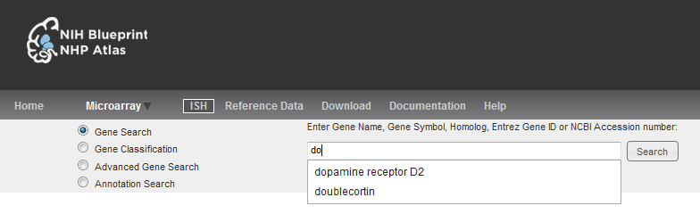
Gene Classification
The ISH data only includes a select number of genes so you can browse the data using the Gene Classification menus. When you land on the ISH Data page, the categories are displayed allowing you to search the genes included for each category.
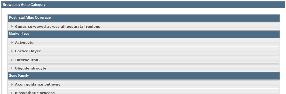
If you are on any other page in the ISH project, click on the “Gene Classification” radio button and select a category from the drop-down menu.
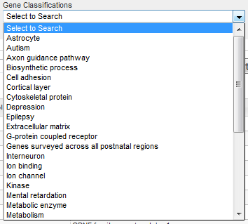
Advanced Gene Search
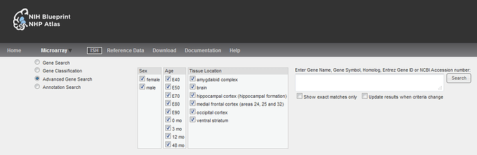
The Advanced Search allows you to narrow your gene search by gender, developmental stage and by tissue location. When you select the “Advanced Gene Search” radio button, you will be able to deselect the categories that don’t pertain to your search. If you do not enter a gene in the search box, all genes that fulfill your search criteria will be returned.
Annotation Search
Experiments conducted on the post-natal stages were manually annotated for their Expression Intensity and their Expression Density.
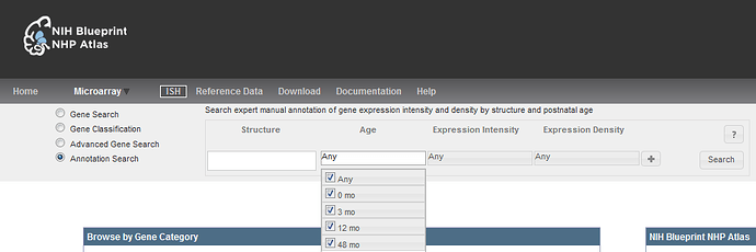
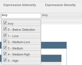
For a detailed description of the manual annotation process, please see the ISH whitepaper in the NHP Documentation. Briefly, both the expression intensity and the expression density were scored on a scale from 1-5.
To perform an annotation search, first choose the brain region or structure of interest from the ontology. Clicking in the Structure search box will open the drop-down menu with all the available structures or regions. Either begin typing your structure into the search box or browse the list in the drop-down. Once you have chosen a structure, choose the developmental stage, the expression intensity and density you are interested in seeing and then click “Search”.
If you would like to include more than one structure in your search, click the “+” button, and repeat the above instructions. If two or more structures (or ages or intensities or densities) are selected in a single row, the search will find all results that match any one of the criteria (i.e. an “OR” search within a row). If more than one row is used, only genes that meet the criteria in ALL rows of the search will be returned (i.e. an “AND” search between rows).
Search Results
Searches will return a list of experiments based on the input search criteria. Each row includes the following information.
| Column | Description |
|---|---|
 | Add the experiment to your selections by clicking the checkbox |
| Experimental ID | Clicking on this link will open the Experimental Details page |
| Gene Symbol (Homolog) | Clicking the Gene Symbol will return Experimental Details pages for all experiments with this gene |
| Gene Name | Full gene name |
| Tissue Location | Tissue location of the sample |
| Age | Ages based on search criteria |
| Specimen ID | Clicking this link will open the Specimen Detail page |
| Donor ID | Allen Institute Donor ID |
| Related Data | Links to other projects conducted with this particular gene |
Sorting
You can sort your results by any any of the columns in either ascending or descending order (by checking the box next to your sort parameter).
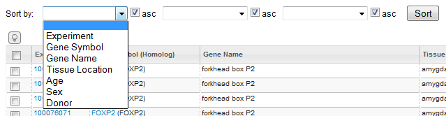
Select the experiments to view in greater detail by clicking on the checkboxes next to your experiments of interest. Experiments will be saved in your cache until you select the “Clear Selections” button at the bottom of the page. After selecting one or more experiments, click the “View Selections” button.
At the bottom of the search results table, there is a link to an XML document containing all of the data in the result set.
Viewing Images
Clicking on the “View Selections” button will open all selected experiments in a new window within individual viewers. The individual experiments can be moved around by clicking and dragging on the title bar and number of columns in this window can be changed by clicking on the gear in the top right-hand corner of the screen.
Zoom and Pan (ZAP) Image Viewer
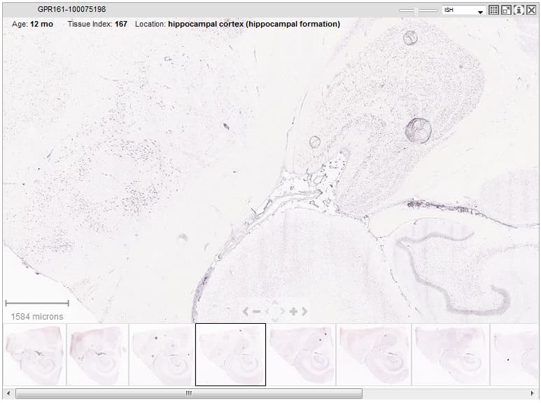
The ZAP image viewer allows you to navigate through an experiment’s images by selecting from one of the thumbnail images along the bottom to select an image to view at higher resolution. The current selection is outlined in black. Once selected, you can Zoom and Pan using the onscreen navigation buttons or use the keyboard commands or the toolbar icons to take additional actions.
The gene symbol or treatment type is displayed in the title bar along with the image series ID. Additional details are displayed across the top of the viewing area, including the age, tissue index and tissue location.
Scale Bar
Shows the current viewing resolution of the image, in microns. This value dynamically changes as you zoom in/out of the image. You can position the scale bar anywhere on the main image by dragging the scale bar by its ruler.
You can toggle the orientation of the scale bar from horizontal to vertical by clicking on the scale bar text.
Keyboard Commands
Toolbar
| Icon | Description |
|---|---|
 | Adjust contrast on the main image |
 | Select ISH, Nissl, or Expression image type |
 | View image series in contact sheet form |
 | Show current image in a High resolution Image Viewer, on its own page |
 | Open a new window to view the Experimental Details Page |
 | Close the current image viewer |
High Resolution Image Viewer
The high resolution image viewer is a viewer that opens in a new window and allows you to get a more detailed view of the experimental images in a structural and cytoarchitectural context.
Side-by-Side Nissl Viewing
Opening the High Resolution Image Viewer will open a new window with your ISH experiment and a side-by-side view of the nearest Nissl image. The left hand viewer shows the ISH image series and the right hand viewer displays the Nissl image series from the same specimen block. By default, the nearest Nissl section to the ISH image you are interested in will be shown and synched with the section you are viewing. Click the “Sync” checkbox to manually correct any synching between the images. Clicking on another ISH image will automatically display its nearest Nissl section. Clicking on an image thumbnail in the Nissl image series will automatically take you to the nearest ISH image. While the “Sync” box is checked the Pan and Zoom functions will affect both ISH and Nissl images.
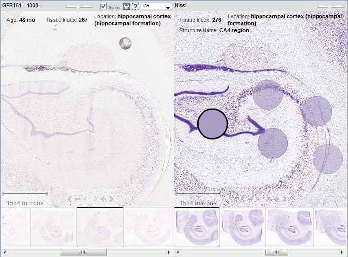
Colored circles in the Nissl slides are hotspots - regions that when moused over list the brain regions manually labeled by our Annotation team.
To download an image, click on the Icon (see below).

Expression Mask Colors
The Expression mask image display highlights those cells that have the highest probability of gene expression using a heat map color scale (from low/blue to high/red).

Experimental Details
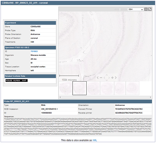
Clicking on the Experiment ID from the search results page or the “i” icon from the image viewers will take you to a page which includes metadata on the experiment, the specimen and the probe as well as related institute data links and a ZAP viewer for all images in the series.
Experiment
This box gives you information on the gene assayed, the probe type and orientation, the plane of section and the kind of treatment (i.e. ISH, Nissl)
Specimen
This box lists the Donor ID in the title bar and lists the Specimen (Clicking this link will open the Specimen Detail information), organism, age, sex, tissue location and hemisphere.
Probe
This box lists the Probe ID in the title bar and includes the type of probe, orientation, NCBI Accession #, GI # and the sequences of the forward and reverse primers so you can recreate this probe for your experiments. It also includes the probe sequence for your reference.
Specimen Detail
Clicking on the specimen link from the search results page or on the specimen link in the experiment details page will take you to detailed specimen information. Specimen detail information includes Specimen Information, Section Information, Gene Information and an Image Viewer.
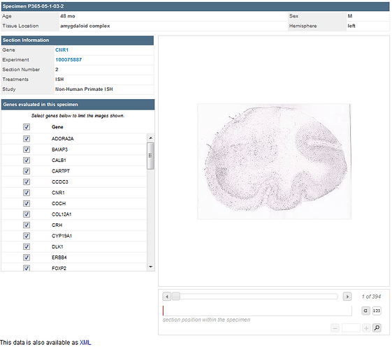
Donor/Specimen Metadata

Specimen ID - internal ID
Age - years
Sex - male or female
Tissue Location - tissue origination in brain
Hemisphere - right or left hemisphere tissue origination
Section Information
The section information box lists information from the current gene pictured in the image viewer including the gene name, the Experiment ID, the section number, the treatment and which study the data came from.
Gene Information
The Gene information section lists the genes that were assayed in this specimen block.
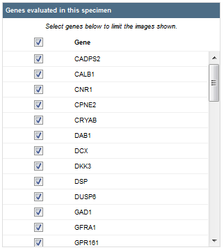
By default, all genes from this specimen are selected for viewing. You can select fewer genes/histological stains to view in the image viewer by first clicking the “Gene” checkbox, then selecting the checkboxes next to the gene/stain(s) you would like to view.
Image Viewer
The viewer displays the image from the current gene listed in the section information box. Below the image, there is an indicator of the position in the specimen block of that particular section, as well as a visualization of the depth of the section into the block. You can view the sections in order (default or by clicking the 123 icon (see below) or grouped by Gene Icon (see below).


When you click on the magnifying glass in the bottom of the image viewer, a new window will open with a magnified view the area in the image viewer outlined by the red box. you can increase or decrease the magnification by clicking the “+” or the “-” buttons.
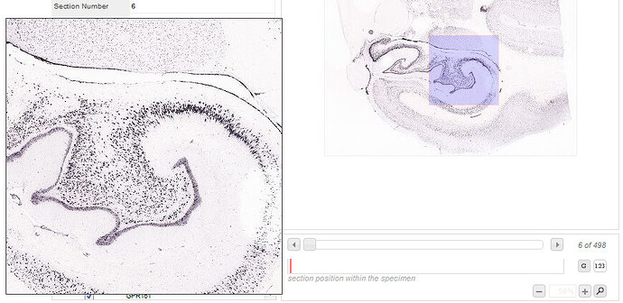
This data can be downloaded as an XML file.
Learn about Allen Brain Explorer Documentation with comprehensive guides and examples from Allen Institute for Brain Science.
Available Files

Learn about Software Development Kit Allen SDK Allen Brain Observatory with comprehensive guides and examples from Allen Institute for Brain Science.
Accessing Allen Brain Observatory data
The AllenSDK is a Python package that facilitates downloading and manipulating Allen Institute data sets. Using the AllenSDK, Allen Brain Observatory experimental data can be retrieved in the Neurodata Without Borders (NWB) file format. The AllenSDK enables deep, custom data analysis by providing utilities for accessing experimental metadata, extracting cell fluorescence traces, and more. It also contains the codebase used to process, quantify, and visualize the data available in Allen Brain Observatory data portal. This includes scripts for:
- neuropil subtraction
- dF/F computation
- stimulus-specific tuning analysis
Getting Started with the AllenSDK
Get started here with the AllenSDK. Users are strongly encouraged to walk through the main Jupyter Notebook for an overview of the available functionality. For example:
Learn about In Situ Hybridization ISH Data For Ivy Glioblastoma Atlas Project with comprehensive guides and examples from Allen Institute for Brain Science.
Searching the Database
Under the ISH tab, there are several ways to search the database.
Specimen Search
To search for a specific glioblastoma specimen type, filter your search criteria by a specific gene, tumor feature, study or specific clinical conditions.

To refine your search by specific clinical conditions, click the “+” next to “Additional Filters By Clinical Conditions”.
If you are unsure of where to begin your search, you can browse by the tumor information where the columns are described below.
Gene Search
The genes chosen for this project were selected based upon current knowledge of GBM biology and what was learned from each of the individual Ivy GAP Studies. To see a list of genes for each study, please see the Gene Lists whitepaper in Documentation. Typing in the gene search text box will bring up a list of suggested genes. If your gene of interest was not assayed in this project, no results will be returned. Once you have chosen a gene, either by selecting a gene from the suggested list, or hitting “Enter” after typing in the name, symbol or ID, a list of specimen blocks that contain search results fulfilling your criteria will open.
Tumor Feature
Each of the tumor structural features was identified and labeled in ~12,000 H&E histological images using a semi-automated annotation application based on advanced statistical machine learning algorithms, and can be searched and visualized in the Ivy GAP web application.
Tumor features are described using a specific ontology. The Ivy GAP ontology is a hierarchical organization of glioblastoma anatomic structural features and associated transcriptomes from RNA-Seq samples that were identified by reference histology or reference gene expression patterns. It does not reflect ontological origins of the structural features; it is simply a representation of relationships among the glioblastoma features and gene expression patterns associated with putative cancer stem cell clusters that were identified in the project.
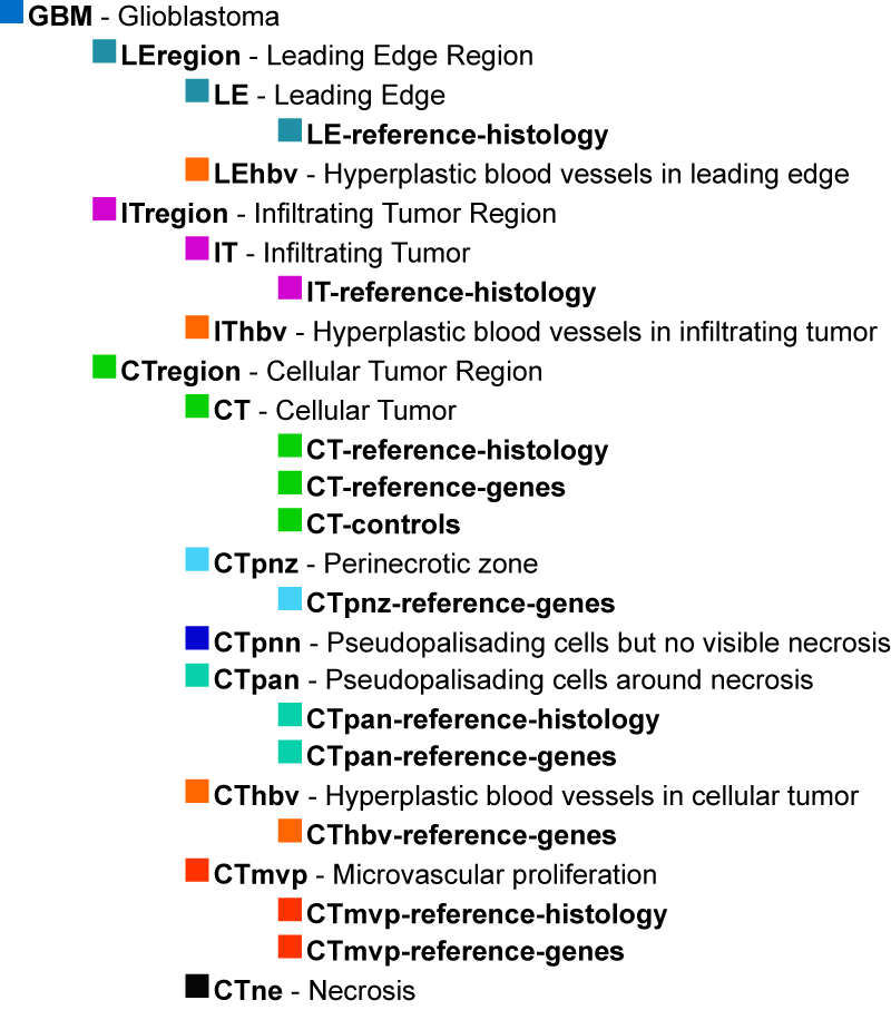
The structural features are commonly identified by neuropathologists in glioblastoma tissue sections stained with Hematoxylin and Eosin (H&E). The major structural regions are Leading Edge (LE), Infiltrating Tumor (IT), and Cellular Tumor (CT).
Within each of these regions, particular structural features can be found such as Microvascular Proliferation (MVP), Pseudopalisading Cells around Necrosis (PAN), Hyperplastic Blood Vessels (HBV), and Necrosis (NE). These features are routinely used to distinguish glioblastoma, or Grade IV glioma, from lower grades of glioma. The feature HBV can be observed occasionally in the LE and IT regions, but it as well as MVP, NE, and PAN are frequently identified in the CT region.
Specimen Search Results
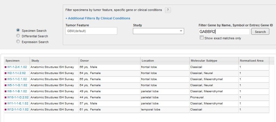
Differential Search
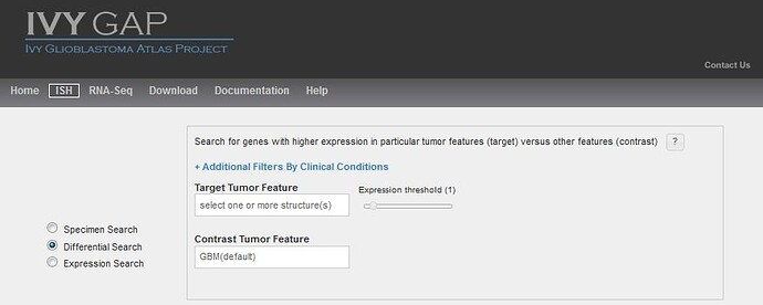
Similar to other Atlases in the Allen Brain Atlas resources, you can search for enriched gene expression in a tumor feature or structure by comparing expression between your target structure and a contrast structure. By default, this search uses all the data as contrast, but changing the contrast structure to more define your search will produce different results. Changing the threshold on a differential search will restrict the list of returned results by excluding any experiment where the expression energy of the target structures is less than threshold.
Several differential searches have already been calculated for you and are accessible by selecting from the “Browse by Differential Expression”.
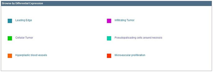
Differential Search Results
Performing a differential search will return a list of specimen blocks that include the genes with the highest differential expression levels ranked by fold change in the target structure over the contrast structure.
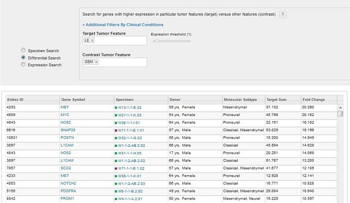
Expression Search
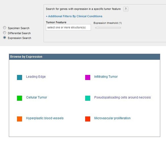
To see gene expression ranked by expression energy within a single glioblastoma structure, use the Expression Search feature. Clicking on a tumor feature from the Glioblastoma Ontology or the “Browse by Expression” box will return a list of genes ranked by the average expression where each column is described below.
Clinical Conditions
When searching for specific images, one of the search tools available to you is to “Filter by Clinical Condition”. Each condition and its significance is outlined below. Listed references can be found in the Overview whitepaper in Documentation.
Molecular Subtype
Genomic characteristics of tissue block related to classification of patients. The molecular subtype was determined using all cellular tumor samples from a given tumor. An analysis of each cellular tumor sample was conducted with 840 transcripts from the RNA-Seq data as per Verhaak et al., 2010. For a given tumor, if multiple cellular tumor samples exhibited distinct subtypes, then the tumor was classified as a mixture of its subtypes. The Classical subtype refers to chromosome 7 amplification, specifically EGFR, paired with chromosome 10 loss. The Mesenchymal subtype is noted for focal hemizygous deletions of a region at 17q11.2, containing the gene NF1. The Proneural subtype is defined by alterations of PDGFRA and point mutations in IDh2. The Neural subtype is typified by the expression of neuronal markers such as NEFL, GABRA1, SYT1, and SLC12A5.
Extent of Resection
Degree to which tumor tissue was surgically removed. Complete resection is associated with increased survival rates (Keles et al., 1999).
Multifocality
Whether a tumor was comprised of single or multiple masses. Increased multifocality is associated with decreased rates of survival (Thomas et al., 2013).
MGMT Methylation
A diagnostic test result referring to whether a tumor’s O-6-methylguanine-DNA methyltransferase DNA repair gene was methylated. Methylated MGMT is associated with increased rates of survival (Hegi et al., 2013).
Survival Days
Patient’s lifespan since initial diagnosis
EGFR Amplification
A diagnostic test result referring to whether a particular tumor’s epidermal growth factor receptor gene had multiple copies. The gene is frequently amplified in glioblastoma (Hobbs et al., 2012).
Initial KPS
Karnofsky Performance Status when first diagnosed with first tumor. Karnofsky Performance Status is a measure of functional impairment on a scale of 0-100, 0 referring to dead, 50 to requiring considerable assistance and frequent medical care, and 100 referring to no evidence of disease. High scores are associated with increased survival rates (Ening et al., 2015).
Age
Patient age in years at time of diagnosis. Younger patients tend to have increased survival rates (Ening et al., 2015).
Specimen Detail Page
Donor Page
Clicking on a Specimen ID will bring you to the specimen detail page.
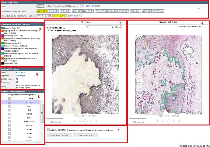
- Tumor Subdivision - Navigation of tumor subdivisions and button for viewing patient and tumor summary information. the color in a tissue sub-block indicates the study in which the sub-block was used.
- Tumor Features in this Sub-Block - The glioblastoma tumor features that were identified and assayed for in the yellow highlighted sub-block. The color coding corresponds to the glioblastoma ontology.
- ISH Image - An image viewer showing the in situ hybridization experiment, and related features.
- Nearest H&E Image - Image and annotated anatomic tumor features of a nearby H&E stained tissue section.
- Section Information - Lists the Gene, Experiment ID, Section #, Treatments, and the study.
- Genes Surveyed in this Sub-Block - All genes assayed in this specimen sub-block are listed. To view a specific gene, select only that gene from the list.
- Selection Cart - When viewing an ISH image, select the checkbox to add the image to your viewing cart. Images selected in your cart are available to view until the cache is cleared or you click “Clear Selections”.
Patient, Tumor and MRI Summary
This panel displays information on patient and tumor, and on how the tumor was subdivided into blocks. This panel is arrived at by toggling the “View Patient, Tumor and MRI Summary” button in the Tumor Subdivision section of the Specimen Detail Page.

Description of Donor ID
The tumor names (or IDs) identify tumors across the different resources associated with the Ivy Glioblastoma Atlas Project. In the name W1-1-2, W1 identifies the patient, and -1-2 indicate that this tumor was the second mass removed during the first surgery.
The names of the tumor blocks were assigned as indicated in the Resected Tumor Image, and the names of the sub-blocks reflect their position within the tumor block.
Image Viewer
The GBM image viewer allows you to navigate through a series of specimen sub-block ISH images to view at higher resolution. Once a gene image is selected, you can manipulate it with your mouse and use the keyboard or on screen navigation tools to take additional actions.
The gene symbol and gene name are displayed in the title bar along with a dropdown menu and a “Sync” feature to allow you to navigate and keep the adjacent H&E viewer synched with your movements. The dropdown menu allows you to view the ISH image, the Expression Mask, the annotated features, or the annotated feature boundaries. If all the genes are selected in Box #6, the entire specimen sub-block can be viewed using the onscreen navigation tools or the keyboard commands. The current selection is outlined in black.
To view images at high resolution, in the Section Information box, click on the Experiment link; then, click the icon in the upper right corner of the viewer. Use the dropdown menu to select the type of image you want to see.
Alternatively, to view all the images available for a given gene, in the Section Information box, click on the gene symbol link.
Scale Bar
Shows the current viewing resolution of the image, in microns. This value dynamically changes as you zoom in/out of the image. You can position the scale bar anywhere on the main image by dragging the scale bar by its ruler.
You can toggle the orientation of the scale bar from horizontal to vertical by clicking on the scale bar text.
Keyboard Commands
Expression Mask Colors
The Expression mask image display highlights those cells that have the highest probability of gene expression using a heatmap color scale (from low/blue to high/red).
Learn about API For Ivy Glioblastoma Atlas Project with comprehensive guides and examples from Allen Institute for Brain Science.
The Ivy Glioblastoma Atlas Project (Ivy GAP) is a foundational resource for exploring the anatomic and genetic basis of glioblastoma at the cellular and molecular levels.
Six studies were designed to identify the molecular signatures and measure heterogeneity. In Situ Hybridization (ISH) was used to screen for gene expression enriched in particular structures and cell clusters, and laser microdissection followed by RNA sequencing were used to generate the transcriptomes and identify the genetic markers.
Overall, the dataset spans 42 individual tumors. Each tumor was sub-divided into sub-blocks for processing in one of the six studies. See whitepapers for more details about the tumor specimens, tissue and informatics processing.
From the API, you can:

Download images
Download quantified ISH expression values by tumor feature

Query the ISH expression differential search services
Download RNA-Seq expression values
Query the RNA-Seq correlative and differential search services
This document provides a brief overview of the data, database organization and example queries. API database object names are in camel case. See the main API Documentation for more information on data models and query syntax.
ISH Surveys
Experimental Overview and Metadata
Experimental data from the four ISH surveys is associated with the “Glioblastoma” Product.
Multiple genes were assayed using each sub-block Specimen. The Specimen is cryosectioned into 20µm thick sections. ISH sections are interleaved with H&E sections such that every ISH is adjacent to an H&E section, yielding a single image SectionDataSet for each gene and one H&E SectionDataSet with 11-15 images.
Each sub-block Specimen is associated with a SpecimenType identifying the study to which this sub-block belongs.
Each H&E section is processed through a semi-automated annotation application that labels anatomic features using a statistical machine learning algorithm. The algorithm associates each 45x45 pixel neighborhood to a tumor feature label. Additionally, a separate algorithm counts the number of nuclei and the nuclei fraction coverage within each neighborhood.
Tumor feature statistics for each sub-block Specimen are generated by summing up the 45x45 pixel neighborhoods over all H&E images. This process produces area, normalized area, nuclei count, and nuclei fraction coverage for each sub-block Specimen and feature of interest.
Anatomic tumor features (also referred to as structures) are hierarchically organized into a tree in which a child structure is a “part of” its parent structure. Structures are assigned colors to visually emphasize their relationships in the hierarchy. See the structure ontology page for more information.
Examples:
- All donors in the “Glioblastoma” Product
http://api.brain-map.org/api/v2/data/query.xml?criteria= model::Donor, rma::criteria,products[name$eq'Glioblastoma']
- All sub-block Specimens which are part of the “Anatomic Structures ISH Survey”
http://api.brain-map.org/api/v2/data/query.xml?criteria= model::Specimen ,rma::criteria,specimen_types[name$eq'Anatomic Structures ISH Survey'] ,rma::options[num_rows$eqall]
- All TumorFeatures in sub-block Specimen “W32-1-1-K.01”
http://api.brain-map.org/api/v2/data/query.xml?criteria= model::TumorFeature ,rma::criteria,data_set(specimen[external_specimen_name$eq'W32-1-1-K.01']) ,rma::include,structure
- All ISH SectionDataSets in sub-block Specimen “W32-1-1-K.01”
http://api.brain-map.org/api/v2/data/query.xml?criteria= model::SectionDataSet ,rma::criteria,specimen[external_specimen_name$eq'W32-1-1-K.01'],treatments[name$eq'ISH'] ,rma::include,genes,sub_images
From the above query, specimen “W32-1-1-K.01” has 21 ISH SectionDataSet (id=278269453 is one of them). In the web application, images from a specimen are displayed in a specimen page. All displayed information, images and structural expression values are also available through the API.
See the image download page to learn how to download images at different resolutions and regions of interest.
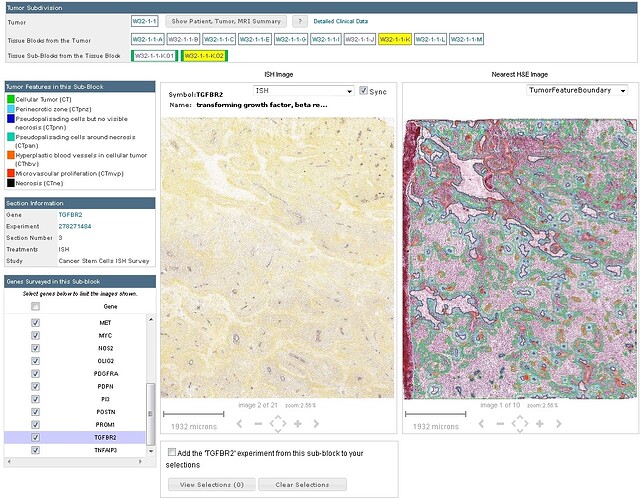
ISH Expression Quantification
For every ISH image, pixels with gene expression are detected and a grayscale mask generated. The detection algorithm is based on adaptive thresholding and mathematical morphology. Then the ISH image is registered to its closet H&E image using a multi-resolution elastic registration algorithm. Finally, feature label and nuclei count information is transferred from 45x45 pixel neighborhood in the H&E image onto the expression data.
Expression statistics for each tumor feature are computed by combining values from all the neighborhoods with the same label. This process produces expression density, intensity and energy measurements for each experiment and anatomical feature. For an anatomical feature, expression energy is defined as sum of expressing pixel divided by sum product of pixels in each neighborhood label for that feature and its nuclei fraction coverage.
Examples:
- Download tumor feature expression values for POSTN SectionDataSet (id=265857641) in sub-block “W8-1-1-E.1.03”
http://api.brain-map.org/api/v2/data/query.xml?criteria= model::StructureUnionize ,rma::criteria,section_data_set[id$eq265857641] ,rma::include,structure
ISH Expression Search Service
The expression search service allows users to instantly search over the ~18000 SectionDataSets to find genes with specific expression patterns:
- The Expression Search function allows users to find genes which expression in one structure (or set of structures)
- The Differential Search function allows users to find genes which have higher expression in one structure (or set of structures) compared to another structure (or set of structures)
The expression search functionality is available through the Web application and the API.
To perform an Expression Search, a user specifies a set of target structures. For each StructureDataSet, the average expression energy is computed for the target structures. The returned results are sorted in descending order of average expression energy.
See the connected service page for definitions of service::gbm_ish_expression parameters
Examples:
- Find genes (SectionDataSets) with expression in pseudopalisading cells around necrosis (CTpan)
http://api.brain-map.org/api/v2/data/query.xml?criteria= service::gbm_ish_expression[structures$eqCTpan][threshold$eq0,100000]
- Find genes (SectionDataSets) with expression in hyperplastic blood vessels (LEhbv, IThbv, CThbv)
http://api.brain-map.org/api/v2/data/query.xml?criteria= service::gbm_ish_expression[structures$eqLEhbv,IThbv,CThbv][threshold$eq0,100000]
To perform a Differential Search, a user specifies a set of target structures and a set of contrast structures. For each StructureDataSet, the sum expression energy is computed for the target structures and for the contrast structures. The returned results are sorted in descending order of the ratio of the sum expression energy of the target structures over the sum expression energy of the contrast structures.
See the connected service page for definitions of service::gbm_ish_differential parameters
Examples:
- Find genes (SectionDataSets) with higher expression in pseudopalisading cells around necrosis (CTpan) than cellular tumor cells (CT)
http://api.brain-map.org/api/v2/data/query.xml?criteria=service::gbm_ish_differential [structures1$eqCT][structures2$eqCTpan][threshold1$eq0,100000][threshold2$eq1,100000]
- Find genes (SectionDataSets) with higher expression in infiltrating tumor (IT) than cellular tumor (CT) and leading edge (LE)
http://api.brain-map.org/api/v2/data/query.xml?criteria=service::gbm_ish_differential [structures1$eqIT,CT][structures2$eqIT][threshold1$eq0,100000][threshold2$eq1,100000]
It should be noted that the expression quantification values used by the search services are generated by a fully automated processing pipeline. False positive and false negative results can occur due to artifacts on the tissue section or slide and/or algorithmic inaccuracies. Users should confirm results by visually inspecting the ISH images.
RNA-Seq Surveys
Experimental Overview and Metadata
Experimental data from the two RNA-Seq surveys is associated with the “Human Glioblastoma RNASeq” Product.
For the “Anatomic Structures RNA-Seq” study, sampling locations were manually identified after H&E staining. For the “Cancer Stem Cells RNA-Seq”, 17 reference gene probes were used to identify 35 types of putative cancer stem cell clusters.
Each sampling site is associated with a Structure with the following naming scheme:
- XX-reference-histology: tumor feature XX sampled by reference histology
- XX-reference-genes: tumor feature XX sampled by reference gene(s)
- XX-reference-controls: tumor feature XX sampled by low expression of reference genes
Structures are organized hierarchically into a tree in which children structures are “parts of” their parent structure. Structures are assigned colors that visually emphasize the hierarchical relationships. See the structure ontology page for more information.
See whitepapers for more details about the RNA-Seq data generation and normalization. All gene and sampling site information can be accessed through the API.
Examples:
- All donors in the “Human Glioblastoma RNASeq” Product
http://api.brain-map.org/api/v2/data/query.xml?criteria= model::Donor, rma::criteria,products[name$eq'Human Glioblastoma RNASeq']
- All samples in the “Human Glioblastoma RNASeq” Product
http://api.brain-map.org/api/v2/data/query.xml?criteria= model::Sample ,rma::criteria,tissue_sample_data_set(products[name$eq'Human Glioblastoma RNASeq']) ,rma::include,structure,tissue_sample_data_set(specimen(donor)) ,rma::options[num_rows$eqall]
RNA-Seq Expression Download Service
Normalized gene-level expression values can be downloaded in several ways:
- From the web application Download page
- From the connected data service in the API
Using the connected service, expression values can be obtained by specifying:
- a list of “probes” (genes),
- a list of “donors” (tumor specimens, optional), and
- a list of structures (optional)
See the connected service page for definitions of service::gbm_expression parameters.
Example:
Download expression values for gene ESM1 restricted to samples from tumor ‘W1-1-2’
- Find Specimen ID for tumor ‘W1-1-2’ (id=703393)
http://api.brain-map.org/api/v2/data/query.xml?criteria= model::Specimen ,rma::criteria,[external_specimen_name$eq'W1-1-2']
- Find Gene ID for human gene ESM1 (id=10924)
http://api.brain-map.org/api/v2/data/query.xml?criteria= model::NcbiGene ,rma::criteria,[acronym$eqESM1],organism[name$eq'Homo Sapiens']
- Use tumor and gene ID as parameters to service::gbm_expression
http://api.brain-map.org/api/v2/data/query.xml?criteria= service::gbm_expression[probes$eq10924][donors$eq703393]
The output of the service has two top level ordered arrays “probes” and “samples”. For example:
“probes”:[{“id”:10924, “name”:“endothelial cell-specific molecule 1”, “gene-id”:10924, “gene-symbol”:“ESM1”,“gene-name”:“endothelial cell-specific molecule 1”, “entrez-id”:11082,“chromosome”:“5”,“start-position”:“n/a”,“end-position”:“n/a”, “expression_level”:[“1.0498”,“0.3790”,“0.1323”,“0.1894”,“0.2724”,“0.0268”,“0.0000”,“1.3249”,“1.0818”,“0.9904”,“1.4085”,“0.0301”,“0.0000”,“0.6687”,“6.9482”,“7.9008”,“6.8374”,“8.5132”], “z-score”:[“-0.6017”,“-0.8612”,“-0.9566”,“-0.9345”,“-0.9024”,“-0.9974”,“0.0000”,“-0.4953”,“-0.5893”,“-0.6247”,“-0.4630”,“-0.9961”,“0.0000”,“-0.7491”,“1.6797”,“2.0481”,“1.6368”,“2.2850”]} ],“samples”:[ {“donor”:{“id”:703393,“name”:“W1-1-2”,“age”:“”,“color”:“646464”},“sample”:{“well”:300629386,“polygon”:298763268,“mri”:[-1,-1,-1]}, “structure”:{“id”:298764274,“name”:“Leading Edge sampled by reference histology”,“abbreviation”:“LE-reference-histology”,“color”:“218FA5”}, “top_level_structure”:{“id”:9429,“name”:“Glioblastoma”,“abbreviation”:“GBM”,“color”:“006EC6”}}, {“donor”:{“id”:703393,“name”:“W1-1-2”,“age”:“”,“color”:“646464”},“sample”:{“well”:300629325,“polygon”:298726093,“mri”:[-1,-1,-1]}, “structure”:{“id”:298764274,“name”:“Leading Edge sampled by reference histology”,“abbreviation”:“LE-reference-histology”,“color”:“218FA5”}, “top_level_structure”:{“id”:9429,“name”:“Glioblastoma”,“abbreviation”:“GBM”,“color”:“006EC6”}}, {“donor”:{“id”:703393,“name”:“W1-1-2”,“age”:“”,“color”:“646464”},“sample”:{“well”:300173638,“polygon”:298727595,“mri”:[-1,-1,-1]}, “structure”:{“id”:298764274,“name”:“Leading Edge sampled by reference histology”,“abbreviation”:“LE-reference-histology”,“color”:“218FA5”}, “top_level_structure”:{“id”:9429,“name”:“Glioblastoma”,“abbreviation”:“GBM”,“color”:“006EC6”}}, … ],
Each probe (Gene) contains information about:
- the Gene (id, name)
- the associated NCBI Gene (id, acronym, name, entrez-id), along with
- a vector of normalized expression values and z-scores in the same order as the “samples” array.
Each sample contains information about:
- the Tumor (id and name returned in the “donor” field)
- the associated Structure (id, name, acronym and color)
RNA-Seq Expression Search Service
Differential Search
The Differential Search finds genes that show the greatest difference in expression values between two sets (target and contrast) of user-defined structures. For each probe, a 2-sample t-test is performed followed by a Benjamini and Hochberg false discovery rate correction. The null hypothesis is that the average expression level of samples in the contrast set of structures is greater than or equal to the average expression level of samples in the target set of structures. A statistically significant result (p-value less than user-defined threshold) allows us to reject the null hypothesis and conclude that the average expression level of samples in the target set of structures is greater than the average expression level of samples in the contrast set of structures. Resulting p-values are sorted in ascending order. Search results can also be sorted by fold-change (log ratio of expression) in descending order.
The differential search functionality is available through the Web application and the API.
See the connected service page for definitions of service::gbm_differential parameters.
Example:
- Differential search for genes with higher expression in microvascular proliferation (sampled by reference histology) than in cellular tumor, infiltrating tumor, leading edge and pseudopalisading cells around necrosis.
http://api.brain-map.org/api/v2/data/query.xml?criteria= service::gbm_differential [structures1$eq'CT-reference-histology','IT-reference-histology','LE-reference-histology','CTpan-reference-histology'] [structures2$eq'CTmvp-reference-histology'][sortby$eq'fold-change']
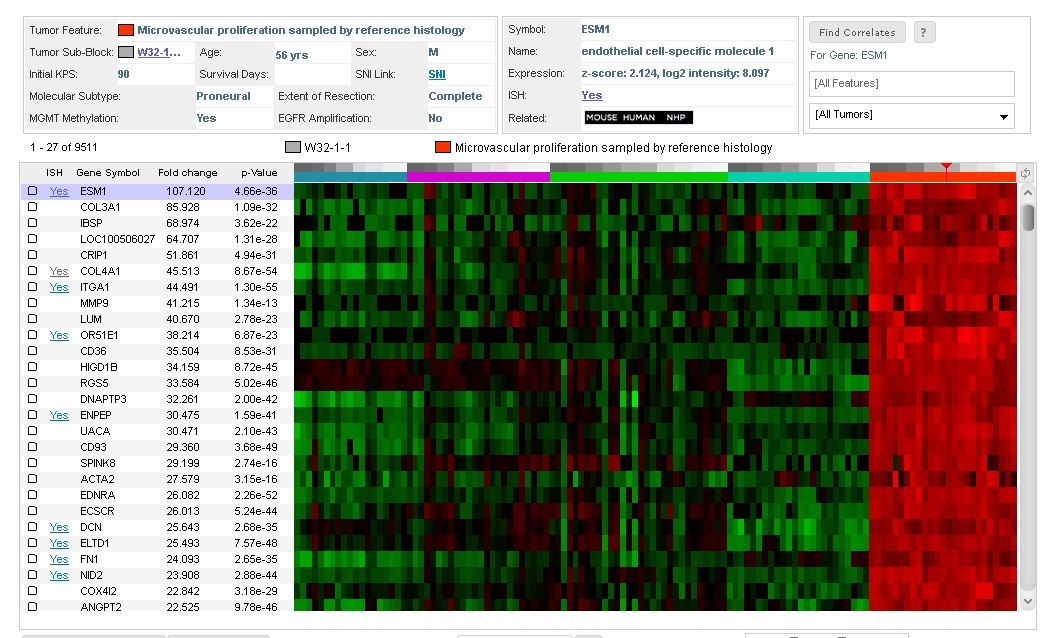
Correlative Search
The Correlative Search finds genes with expression profiles similar to that of a selected seed “probe” over all samples within a user-specified structure and for user-specified tumors/donors. Pearson’s correlation coefficients are computed for all probes and the results ranked in descending order.
The correlative search functionality is available through the Web application and the API.
See the connected service page for definitions of service::gbm_correlation parameters.
Example:
- Correlative search for genes with a similar expression to gene VEGFA (id=7379) over all samples
http://api.brain-map.org/api/v2/data/query.xml?criteria= service::gbm_correlation[probes$eq7379][structures$eqGBM]Learn about Brainspan In Situ Hybridization ISH Data with comprehensive guides and examples from Allen Institute for Brain Science.
Gene Search
To search for a specific gene or group of genes, type its gene name, gene sympol, NCBI Accession number, or Entrez Gene ID into the search box. Make sure the Gene radio button is selected and click the “Search” button. You will be offered suggestions to choose from while you type, but you can also search by typing the first three or more letters in its name or symbol and appending an asterisk ( * ) as a wildcard. You can also browse through the genes by clicking on a category.
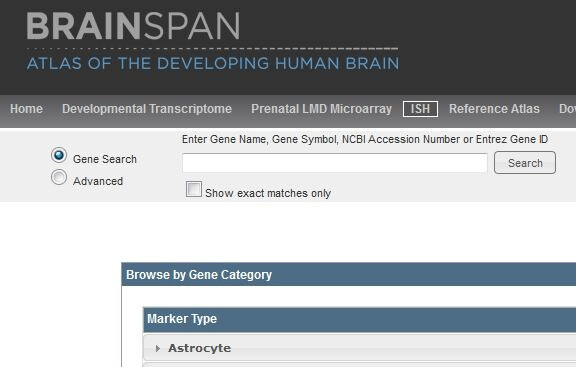
You can sort the search results or further refine your query using the Advanced Search feature.
Advanced Search
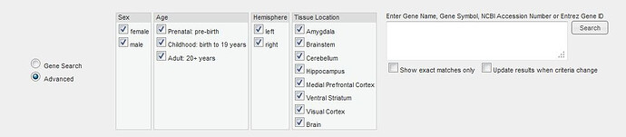
Several additional search criteria can be used to build a query using “Advanced Search.”
The following search criteria can be specified in the text box to the right of the categories. If you copy + paste in a list of terms delimited by tabs or carriage returns they will automatically be converted into a list of search criteria separated by the OR operator ( | ).
- Gene symbol
- Gene name
- Gene aliases
- Entrez gene ID
Boolean Syntax
The following special operators can be used to build queries:
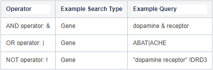
- AND, OR and NOT may be used in place of their corresponding operators. They must be upper case.
- The AND operator (&) is implicit, so spaces between words that are not separated by an operator will be treated like an &.
- OR (|) has higher operator precedence than AND (&).
- Parenthesis can be used to group criteria, but nested parenthesis are not supported at this time.
- The NOT operator (!) is not supported within parenthesis.
- Enclose search terms in quotation marks to avoid confusion with boolean operators. For example, hyphenated words should be enclosed in quotation marks (i.e. “ATP-binding”).
Search Results
Based on your search criteria, a list of experiments will be returned as described in the table below. Search results can be sorted by up to three categories indicated by the drop down menus. Search categories are prioritized from left to right and include all searchable columns. The checkbox labeled “asc” (ascending order)indicates the sorting direction for each column, so when checked, the sort progresses from a to z , or 1 to n, depending on whether the column is alphabetic or numeric. Leaving the box unchecked sorts the column in descending order, that is z to a, or n to 1.
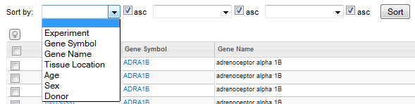
ISH - Image Viewing
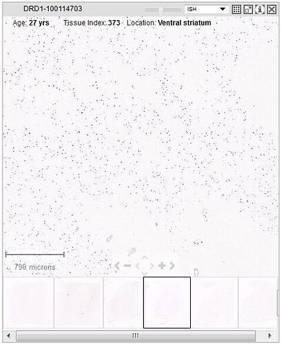
The Zoom and Pan (ZAP) Image Viewer window allows you to view the images from one or more experiments once they have been selected from the search returns list (by clicking the checkbox(es) and clicking “View Selections”). Each ZAP viewer consists of a filmstrip of thumbnails - which when selected will bring up the image in the main viewer, tools to navigate the image in the main viewer and a scale bar to determine the approximate size of the area in the main viewer.
To alter your workspace, click on the selections wheel at the top left hand corner of the ZAP Viewer window to select the number of columns (i.e. the number of experiments you can fit across the page).
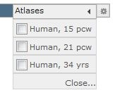
The size of your viewers will automatically adjust to fit your screen real estate. Selecting one of the references from the Atlas drop down menu will allow you to see an annotated reference atlas along side your experiments. Drag viewers to other positions to rearrange them.
The gene symbol or treatment type is displayed in the title bar along with the Allen Institute image series ID. Additional details are displayed across the top of the viewing area, including the donor age, tissue index, and tissue location.
Thumbnails for the entire image series are displayed across the bottom of the viewer in section order. Click a thumbnail to select it for viewing, or use the keyboard to navigate through the set. The current selection is outlined in black.
Toolbar

Scale Bar
Shows the current viewing resolution of the image, in microns. This value dynamically changes as you zoom in/out of the image. You can position the scale bar anywhere on the main image by dragging the scale bar by its ruler.
You can toggle the orientation of the scale bar from horizontal to vertical by clicking on the scale bar text. When you download an image, the scale bar is not included with the image.
Side By Side Nissl Viewing
Once you click on the full screen viewer button, you will be taken to a screen with side by side viewers. The left hand viewer shows the ISH image series and the right hand viewer displays the closest Nissl image from the same specimen block. Clicking on another ISH image will automatically display its nearest Nissl section. Clicking on an image thumbnail in the Nissl image series will automatically take you to the nearest ISH image. While the “Sync” box is checked the Zoom and Pan functions will affect both images. Round spots on the Nissl image are “hotspots” and when hovered over will display the name of the structure. Clicking on the hotspots while viewing ISH images from an adult brain will take you to the Adult Human ISH Guide. While viewing pre-natal ISH images, clicking on the hotspot will take you to the appropriate aged prenatal Reference Atlas.

Keyboard Commands
Expression Mask Colors
The Expression Mask image display highlights those cells that have the highest probability of gene expression using a heat map color scale (from low/blue to high/red).
Experiment Details Page
Clicking on the experiment ID from the search results page will return a page with metadata about the experiment including experiment details, specimen details, related Institute data, probe details and a ZAP Image Viewer.

Gene Details Page
When you click on the the gene symbol from the search returns page you will be taken to a page that includes all the experiments performed in this study with this gene.
Specimen Detail Information
Clicking on the specimen link from the search results page or on the specimen link in the experiment details page will take you to detailed specimen information. Specimen detail information includes Specimen Information, Specimen Block Layout, Section Information, Gene Information and an Image Viewer.
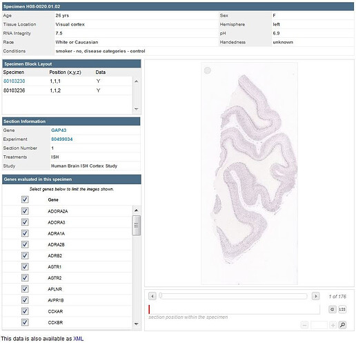
Donor/Specimen Metadata

Specimen ID - internal ID
Age - years
Sex - male or female
Tissue Location - tissue origination in brain
Hemisphere - right or left hemisphere tissue origination
RNA Integrity Number - metric indicating RNA integrity from tissue. Ranges from 1 to 10 (degraded to intact RNA)
pH - tissue sample pH
Race - ethnicity
Handedness - right, left, or ambidextrous
Conditions - disease conditions, smoker
Specimen Block Layout
Specimens are received as variable sized blocks of frozen tissue. Before they are sectioned for ISH experiments they are divided into a number of sub-specimens. Throughout this site, when we refer to a specimen we are actually referring to one of these sub-specimens.
This list denotes the current sub-specimen (in black) and sibling sub-specimens, with their locations and whether data was collected on the sub-specimen. Sibling sub-specimen can be viewed if there is data (denoted by Y) by clicking on their links.
Section Information
The section information box lists information from the current gene pictured in the image viewer including the gene name, the experiment ID, the section number, the treatment and which study the data came from.
Gene Information
The Gene information section lists the genes that were assayed in this specimen block
By default, all genes from this specimen are selected for viewing. You can select fewer genes/histological stains to view in the image viewer by first clicking the “Gene” checkbox, then selecting the checkboxes next to the gene/stain(s) you would like to view.
Image Viewer
The viewer displays the image from the current gene listed in the section information box. Below the image is an indicator of the position in the specimen block of that particular section, as well as a visualization of the depth of the section into the block. You can view the sections in order (default or by clicking the 123 button (see below)) or grouped by gene (see below)


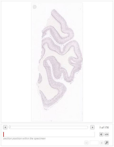
When you click on the magnifying glass in the bottom of the image viewer, a new window will open with a magnified view the area in the image viewer outlined by the red box. you can increase or decrease the magnification with the scale at the bottom.
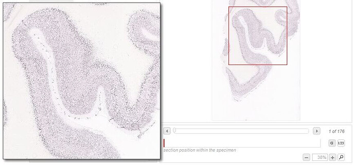
This data can be downloaded as an XML file.
Learn about Documentation Brain Observatory with comprehensive guides and examples from Allen Institute for Brain Science.
Available Files

Learn about Reference Data For NHP Atlas with comprehensive guides and examples from Allen Institute for Brain Science.
Postnatal Reference Series
A set of developmental stage-specific reference series consisting of Nissl histology and magnetic resonance imaging (MRI) to provide neuroanatomical context for the developing macaque brain.
For more information, see the Reference Series technical white paper.
Prenatal Microdissection Microarray: Supporting Data
A set of supporting data consisting of ENC1 and GAP43 ISH staining, Nissl staining and AchE staining of select developmental stages to assist in neuroanatomical delineations.
For more information, see the Microarray Analysis technical white paper.
Learn about Brainspan Searching The Developmental Transcriptome with comprehensive guides and examples from Allen Institute for Brain Science.
The Developmental Transcriptome search functionality can be found by clicking the corresponding button in the menu bar.
Three search types are available: (1) Gene Search, to obtain gene expression data for specific genes of interest, (2) Differential Search, to compare expression between two sets of brain structures at desired developmental stages, and (3) Correlative Search, to find genes that have an expression pattern similar to a “seed gene” selected from the results of a Gene or a Differential search.
Clicking on the “?” button from any search type will take you to the appropriate help section.
Gene Search
With the Gene Search radio button selected (default) you can either select a category from the tag cloud or type the name of your gene of interest into the text box and then click Search. With the October 2013 release, sequence data from non-coding regions was also added to the data-base. You can find that data by entering the ncRNA Ensembl ID.
Results will be returned in a heat map format with the genes on the y-axis (vertical) and the donors/structures on the x-axis (horizontal). The heat map represents the normalized gene level RNA-Seq expression data in RPKM (Reads Per Kilobase of exon model per Million mapped reads). By default, the columns in the heat map are sorted first by donor, then by structure. To toggle the initial sort parameter, click the toggle button in the top right hand corner of the heat map.
Clicking on a data point in the heat map will bring up more information in the panel above the heat map. This information includes the structure (click to be taken to the reference atlas) and donor information, gene information including gene name and symbol (Click to be taken to the exon level data), Ensembl ID, gene expression (in log2 RPKM) and a link to related data in other Allen Brain Atlas resources.
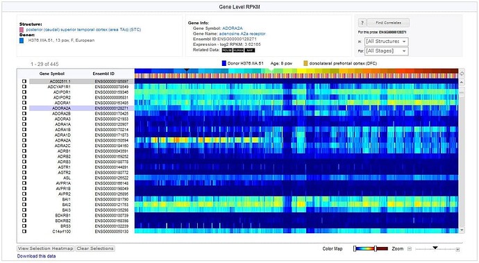
You can adjust the window and the level of the color scale on the heat map by adjusting the threshold bars or re-centering the color map scale bar. You can also zoom in or out to see the heat map at different magnification levels.
You can select a set of probes for later use by selecting the check-boxes beside the list of gene symbols. Your choices are stored in a browser cookie in your computer and will remain in effect until you click the “Clear Selections” button or clear your web browser’s cookie cache. Click the “View Selections” button to see your selections.
Differential Search
Another common usage of gene expression databases is to find genes that show enrichment of expression in one set of samples compared to another set of samples. This type of query is supported by the “Differential Search” mode. Select the “Differential Search” radio button. To find genes enriched in one “target set” of brain regions and/or developmental stages compared to a “contrast set” of brain regions and/or stages, choose the target set using the “Target Structure(s)/Stage(s)” drop down menu, and the contrast set using the “Contrast Structure(s)/Stages(s)” drop down menu. The default setting selects all structures and stages, but clicking on the “All Structures” or “All Stages” drop down menu will allow you to select individual structure(s)/stages(s). Then click “Search”.
The search will return a list of genes enriched in the target domain over the contrast domain. To see only the domains selected from your search criteria, select the “Filter Heatmap” button below the heatmap.
Once selected a window will open allowing you to select the structures and the developmental stages you are interested in visualizing.

Once you have identified a single gene and want to dig deeper into the exon level expression data, click on the blue colored gene name or symbol above the heat map. This link takes you to the transcriptome visualization page.
Correlative Search
In using gene expression databases, a “search by example” feature is also highly desirable as genes with similar expression patterns may be related in function. Using the “Find Correlates” search utility will accomplish this function. This search by example facility is also available in the Allen Human Brain Atlas as well as in the Allen Mouse Brain Atlas and in the Allen Developing Mouse Brain Atlas.
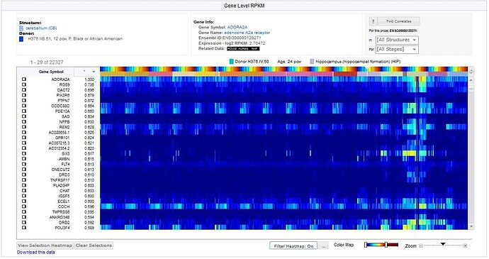
Once you have selected a gene of interest (by clicking on the heat map that results from a Gene or Differential search), you can find genes with similar expression patterns over the entire dataset or over a subset of structures and developmental stages. These subsets can be chosen using the drop down menus. All structures are checked by default, but clicking “All Structures” a second time will deselect all structures, similarly for “All Stages”. Once you have selected the brain region(s) and development stage(s) of interest, click “Find Correlates”.
The search will return a list of genes enriched in the target domain over the contrast domain. To see only the domains selected from your search criteria, select the “Filter Heatmap” button below the heatmap.
Once selected a window will open allowing you to select the structures and the developmental stages you are interested in visualizing.
Once you have identified a single gene and want to dig deeper into the exon level expression data, click on the blue colored gene name or symbol above the heat map. This link takes you to the transcriptome visualization page.
You can see “anti-correlated” genes by toggling the sort order on column “r” or scrolling to the bottom of the heat map.
Download Search Results
To download your search results, click the “Download this data” link at the bottom left of the heatmap. You will have the option of downloading up to 2000 genes at a time starting from any position in the heatmap. Your start position can be determined from the counter in the top left corner of the heatmap (see screenshot).
Your data will be downloaded as three separate files: 1) a Columns.csv file that lists the column headers with associated metadata for each sample, 2) a Rows.csv file that lists the row headers with associated metadata for each gene, and 3) an Expression.csv file that provides a matrix of the expression values for each data point.
The column headers, row headers and expression data will be consistent with the settings from which you downloaded the heatmap (i.e. color map).
Data Visualization
The transcriptome visualization page is divided into 3 sections.
The first section contains gene Information data including the Ensembl symbol and ID, the chromosome number, the NCBI Entrez symbol, ID and name, gene aliases, links to the USC and the Ensembl genome browsers which take you directly to gene locus data, and links to related data from other Allen Brain Atlas resources.

The second section provides a composite gene model where exons are represented by boxes and introns are represented by the green lines between exons. When you hover your mouse over an exon in either the RNA-Seq or exon array data, the exon is highlighted in this model.

The third section contains two tabs:
A tab labeled RNA-Seq with a heat map of the exon level expression data in RPKM (Reads Per Kilobase of exon model per Million mapped reads).
A second tab labeled Exon Array with a heat map of the exon probeset level expression data in log2 transformed normalized expression intensity values.
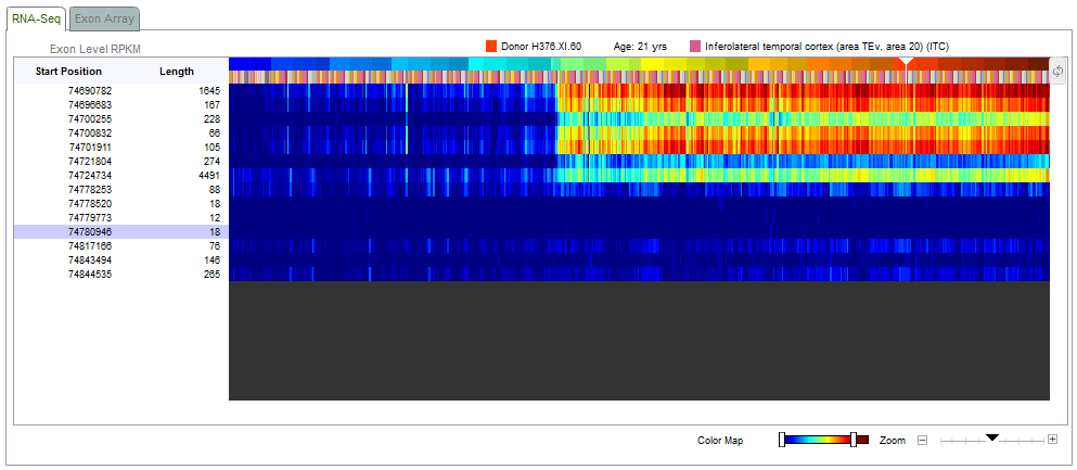
This data can be downloaded by clicking on the “Download this data” link at the bottom left of the heatmap.
Transcriptome Heat Maps
The heat map is a visualization of the exon expression values for the returned gene of interest. The heat map data is presented as a matrix with brain structure (by developmental stage) on the x-axis and gene exons on the y-axis. Brain structures are organized in ontological order. Clicking on the toggle button in the right hand corner will toggle the initial sorting parameter from structure to developmental stage.
Each row of the heat map in the RNA-Seq data represents an exon. Exons in the RNA-Seq data are labeled by the start position on the chromosome and the length of the exon. Each row of the heat map in the Exon Array data represents an exon probeset. Approximately 4 probes are selected for each putative exon region and called a probeset. Each row in the Exon Array data is labeled with the chromosome start position and the length of the probeset. Hovering the mouse over the exon in either heat map will highlight the corresponding exon in the composite gene model over the array data.
Each column of the heat map represents a tissue sample. The colors of the heat map are expression values, transformed to a log 2 scale. The color scale ranges from dark blue representing low expression and passes through cyan, yellow, orange and finally to dark red representing high expression. Hovering the mouse over a cell of the heat map will bring up donor and structure information in the area above the heat map.
Learn about Rna Sequencing Data For Ivy Glioblastoma Atlas Project with comprehensive guides and examples from Allen Institute for Brain Science.
Three search types are available: (1) Gene Search, to obtain gene expression data for specific genes of interest, (2) Differential Search, to compare expression between two sets of glioblastoma anatomic structures, and (3) Correlative Search, to find genes that have an expression pattern similar to a “seed gene” selected from the results of a Gene or a Differential search.
Clicking on the “?” button will take you to the appropriate help section.
Gene Search
With the Gene Search radio button selected (default), you can either select a gene only by typing the name of your gene of interest into the text box, or you can further restrict your selection criteria by selecting tumor features and/or tumors. Once you have made your selections, click the Search button. The search will not work unless a gene has been selected. You can further limit your search by selecting the box next to “Show exact matches only”.

Results will be returned in a heatmap format with the genes on the y-axis (vertical) and the tumors/tumor features on the x-axis (horizontal). The heatmap represents the normalized gene level RNA-Seq expression data in FPKM (Fragments Per Kilobase Of Exon Per Million Fragments Mapped). By default, the columns in the heatmap are sorted first by tumor, then by tumor feature. To change sort order, click the toggle button in the top right hand corner of the heatmap.
Clicking on a data point in the heatmap will populate the metadata box above the heatmap with information specific to that gene and tumor. This meta-information includes information regarding the tumor, the gene and a search box to search for genes that show similar expression patterns as your gene of interest. There are two links available from the tumor box, clicking on the “Tumor Sub-Block” link will open up a new tab with the Specimen Detail Page and clicking the “SNI” link will take you to the Swedish Neuroscience Institute page (registration is required to access the patient metadata). Gene information includes metadata on the gene selected including links to ISH data for that gene (when available) and links to other Allen Brain Atlas resources that include that gene.
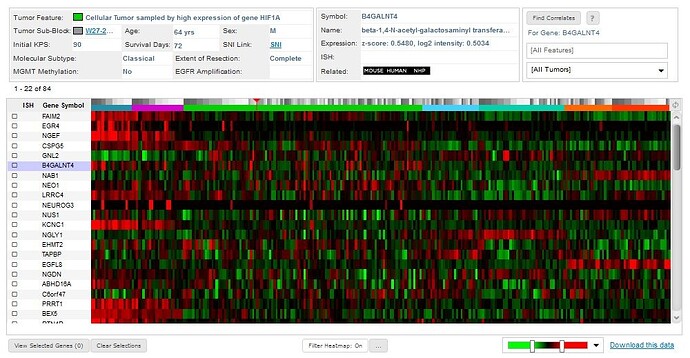
If there is ISH data available for a gene, there will be a link labeled “Yes” that will take you to the ISH Data for that gene.
You can adjust the window and the level of the color scale on the heatmap by adjusting the threshold bars or re-centering the color map scale bar. You can also zoom in or out to see the heatmap at different magnification levels.
You can select a set of genes for later viewing by selecting the check-boxes beside the list of gene symbols. Your choices are stored in a browser cookie in your computer and will remain in effect until you click the “Clear Selections” button or clear your web browser’s cookie cache. Click the “View Selections” button to see your selections.
To restrict the columns that are displayed, select the “Filter Heatmap” button below the heatmap. Filtering your heatmap is a two-step process: first, select the “…” box to restrict your features, making sure to save your selections and then toggle the filter heatmap feature by clicking the “Filter Heatmap” button.
Correlative Search
In using gene expression databases, a “search by example” feature is highly desirable as genes with similar expression patterns may be related in function. Using the “Find Correlates” search utility will accomplish this function.
Once you have selected a gene of interest (by clicking on the heatmap that results from a Gene Search or Differential Search), you can find genes with similar expression patterns. All Features and All Tumors are included in your search by default, but you can select one or more features or tumors from the drop down menus. Once you have selected the tumor feature(s) and tumor(s) of interest, click “Find Correlates”.
The search results highlight the genes whose expression profiles across the samples of interest resemble the expression profile of the example gene by ranking the genes according to the Pearson’s correlation coefficient (r) between their profile and that of the example gene.
If there is ISH data available for a gene, there will be a link labeled “Yes” that will take you to the ISH Data for that gene.
You can adjust the window and the level of the color scale on the heatmap by adjusting the threshold bars or re-centering the color map scale bar. You can also zoom in or out to see the heatmap at different magnification levels.
You can select a set of genes for later viewing by selecting the check-boxes beside the list of gene symbols. Your choices are stored in a browser cookie in your computer and will remain in effect until you click the “Clear Selections” button or clear your web browser’s cookie cache. Click the “View Selections” button to see your selections.
To restrict the columns that are displayed, select the “Filter Heatmap” button below the heatmap. Filtering your heatmap is a two-step process: first, select the “…” box to restrict your features, making sure to save your selections and then toggle the filter heatmap feature by clicking the “Filter Heatmap” button.
You can see “anti-correlated” genes by toggling the sort order on column “r” or scrolling to the bottom of the heatmap.
Differential Search
Another common usage of gene expression databases is to find genes that show enrichment of expression in one set of samples compared to another set of samples. This type of query is supported by the “Differential Search” feature. Under the RNA-Seq tab, click on the examples in the “Browse by Differential Expression” box, or select the “Differential Search” radio button to start your own search. To find genes enriched in one “target set” of tumor features and/or tumors compared to a “contrast set” of tumor features and/or tumors, choose the target set using the “Target Tumor Features/Tumors” drop down menu, and the contrast set using the “Contrast Tumor Features/Tumors” drop down menu. The default setting selects all tumor features and tumors, but clicking in the “All Features” or “All Tumors” text boxes will allow you to select individual tumor feature(s)/tumor(s). Then, click “Search”.

The search will return a list of genes enriched in the target domain(s) over the contrast domain(s) ranked by the Fold change in expression values. The results can be sorted also by the statistical significance of the evidence (p-Value) by clicking on the desired sort parameter.
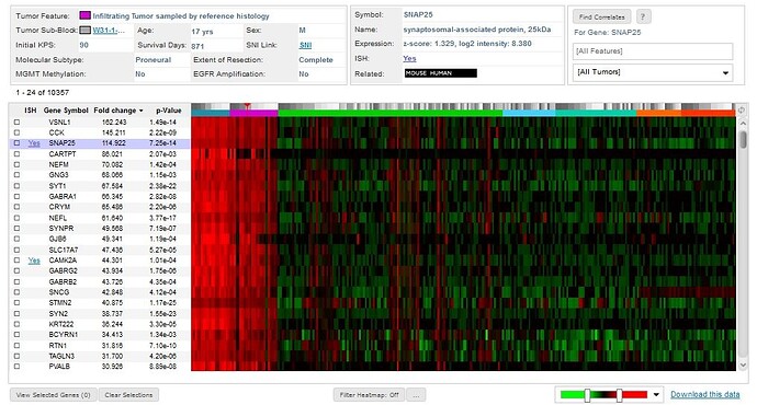
If there is ISH data available for a gene, a link labeled “Yes” takes you to the ISH Data for that gene.
You can adjust the window and the level of the color scale on the heatmap by adjusting the threshold bars or re-centering the color map scale bar. You can also zoom in or out to see the heatmap at different magnification levels.
You can select a set of genes for later viewing by selecting the check-boxes beside the list of gene symbols. Your choices are stored in a browser cookie in your computer and will remain in effect until you click the “Clear Selections” button or clear your web browser’s cookie cache. Click the “View Selections” button to see your selections.
To restrict the columns that are displayed, select the “Filter Heatmap” button below the heatmap. Filtering your heatmap is a two-step process: first, select the “…” box to restrict your features, making sure to save your selections and then toggle the filter heatmap feature by clicking the “Filter Heatmap” button.
Download Search Results
To download your search results, click the “Download this data” link at the bottom left of the heatmap. You will have the option of downloading up to 2000 genes at a time starting from any position in the heatmap. Your start position can be determined from the counter in the top left corner of the heatmap (see screenshot).
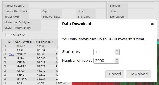
Your data will be downloaded as three separate files: 1) a Columns.csv file that lists the column headers with associated metadata for each sample, 2) a Rows.csv file that lists the row headers with associated metadata for each gene, and 3) an Expression.csv file that provides a matrix of the expression values for each data point.
The column headers, row headers and expression data will be consistent with the settings from which you downloaded the heatmap (i.e. color map).
To download the complete data set used in the heatmap, go to the Download tab and click the appropriate link.
Learn about Documentation For NHP Atlas with comprehensive guides and examples from Allen Institute for Brain Science.
Available Files
Learn about Documentation Ivy Glioblastoma Atlas Project with comprehensive guides and examples from Allen Institute for Brain Science.
Available Files
Learn about Brainspan Downloading Data with comprehensive guides and examples from Allen Institute for Brain Science.
Supplemental Data
The download page allows you access to supplementary data associated with the BrainSpan Atlas of the Developing Human Brain.
Developmental Transcriptome Dataset
Downloadable archive files containing normalized expression values and meta-data (as displayed in heatmap) for analysis:
RNA-Seq Gencode v10 summarized to exons
RNA-Seq Gencode v10 summarized to genes
Exon microarray summarized to probe sets
Exon microarray summarized to genes
Archived data files containing normalized RPKM expression values employing a historical normalization method (available prior to October 2013):
RNA-Seq Gencode v3c summarized to exons
RNA-Seq Gencode v3c summarized to genes
For detailed descriptions of current and historical normalization processes, see the technical white paper,
Prenatal LMD Microarray Dataset
Downloadable archive files containing normalized expression values for each brain and meta-data for analysis:
H376.IIIA.02, male, 15 pcw
H376.IIIB.02. female, 16 pcw
H376.IV.02, female, 21 pcw
H376.IV.03, female, 21pcw
Download XML or CSV containing tissue sample meta-information and URL to download each of the raw LMD microarray files.
3-D Fiber Tract and Developmental Transcriptome Sampling Annotation
3-D expert annotation of 22 major fiber tracts across 8 developmental stages accompanied by annotation of the Developmental Transcriptome survey sampling sites.
14 pcw annotation: fiber tracts , structures
17 pcw annotation: fiber tracts , structures
19 pcw annotation: fiber tracts , structures
37 pcw annotation: fiber tracts , structures
3 yrs annotation: fiber tracts
8 yrs annotation: fiber tracts
15 yrs annotation: fiber tracts
32 yrs annotation: fiber tracts
Supplemental Data
MRI/DTI data for prenatal specimens
Methylation
MicroRNA
MRF bigWig Gencode v10
MRF Gencode v3c
Learn about Rna Sequencing Of The Aging Dementia And TBI Project with comprehensive guides and examples from Allen Institute for Brain Science.
To complement the protein quantification and histological analysis of tissues from this cohort, RNA Sequencing was run on 377 samples taken from cortical grey (parietal and temporal) and white matter (parietal) and hippocampus, with a minimum of 30M 50bp paired-end reads per sample.
Searching
Searching is available using three methods: (1) Gene Search, when looking for a specific gene of interest, (2) Differential Search, to find enhanced gene expression when comparing different brain regions and donors and 3) Correlative Search, to find regions and donors that exhibit similar gene expression to a “seed gene” selected from the results of a Gene or a Differential search.

To browse curated differential searches, click on the desired search term from the RNA-Seq landing page.
Gene Search
When searching for a specific gene of interest, type the unique identifier into the “Filter by Gene Name, Gene Symbol or Entrez Gene ID” text box and either hit enter or click “Search”. You can also narrow your search by selecting a brain region(s) and/or filtering by donor. Default searches query over all donors and all regions. Your search results will open in a heat map viewer.

Differential Search
Without a specific gene marker to initiate your search, a differential search can be useful in that it will look for genes enhanced in the brain region or donor you are interested in. To perform a differential search, you must select target and contrasting brain regions and donors. Select one or more brain regions from the drop-down menus. Filtering by donors requires selecting from the matrix that opens when you click in either text box. The toggle switch to the right of the text boxes will exchange the Target and Contrast selections.
Once you have selected your search criteria, clicking “Search” will open up your results in a heatmap viewer.
Donor Selection
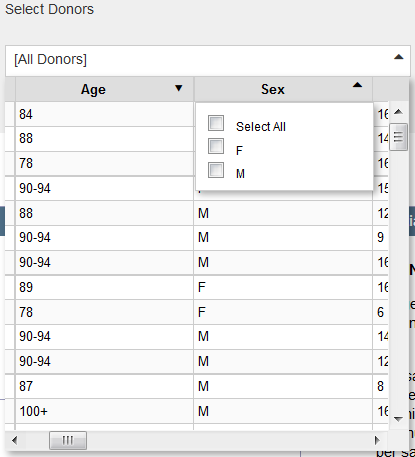
Each of the different search methods provides an opportunity to limit the donors based on metadata collected in the study. To filter the data, click in the text box associated with donor choice to open a matrix. Filter the parameters by selecting the arrow in the column headers to choose parameters. Filter parameters are listed in the table below. For more information regarding the data collected on this cohort, please see the ACT Cohort whitepaper in Documentation.
Search Results
Once you have conducted a gene or differential search or have selected one of the curated searches, your results will be loaded into a heatmap viewer. Once you have clicked on a data point in the heat map, metadata will be populated in the summary above the heatmap.
Metadata Summary

The metadata summary outlines several of the donor categories, metadata on the gene (including symbol, name, expression values and related data) and the find correlates and Genome Browser functions.
Heatmap Viewer
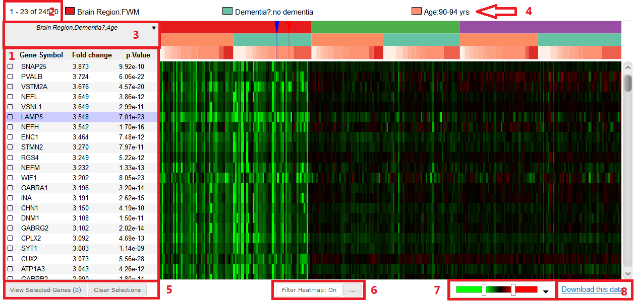
- Gene List: List of genes defined by the search criteria by gene symbol. When the list is a result of a differential search, each gene will be accompanied by both a “Fold Change” and “p-value”. Selecting those column headers will toggle the gene list to that parameter. When the list is the result of a correlative search each gene will be accompanied by a Pearson’s correlation, r.
- Number of Genes: Number of genes that fit the search criteria.
- Column Headers: Clicking in this box will allow you to change the initial sort parameters of the column headers
- Classification: Indicates the column headers consistent with the currently highlighted data point (where the mouse is hovering)
- Gene Selection: Select genes by clicking on the checkbox next to the gene symbol in the gene list. View a heatmap with only selected genes by clicking “View Selected Genes”. Genes will be available for viewing until you click “Clear Selections” or clear your cache.
- Filter Heatmap Function: To limit the amount of data displayed in the heat map use this function.
- Color Map: Use this function to change the way the z-scored data is displayed or to view the log2 FPKM data.
- Download: This link initiates download of the current heatmap data.
Column Sorting

The column headers on the x-axis of the heat map are a feature that can be changed by the user. By default, the column headers are Brain Region, Dementia? and Age (in that order), but any of the donor parameters can be used to sort the columns. Clicking the arrow in the box in the upper left-hand corner of the heatmap will open a list of groupings including any customized groupings that the user has created. To create a new grouping, click on “[Create new grouping…]”, and a window will open allowing you to create a new grouping. Remember to save your selection.
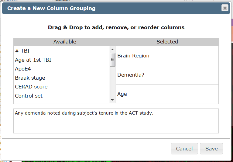
To remove a grouping, hover the mouse over the grouping and a garbage can will appear, click the can to remove the grouping.
Filter Heatmap
To restrict the amount of data that are displayed in the heatmap, select the “Filter Heatmap” button below the heatmap. Filtering your heatmap is a two-step process: first, select the “…” box to restrict your features, making sure to save your selections, and then toggle the filter heatmap feature between “On” and “Off” by clicking the “Filter Heatmap” button.
Download Heatmap Data
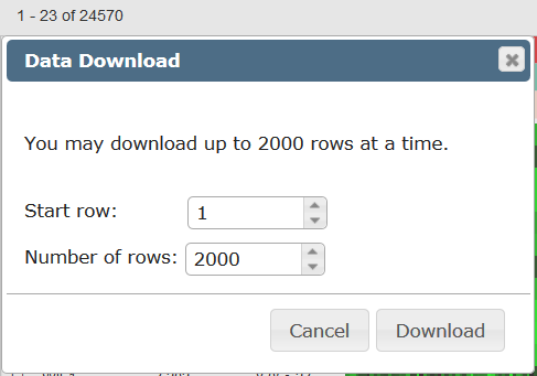
Once you have found the data that you are interested in downloading and analyzing off-line, click on the “Download this data” link. There is a limit to the amount of data you can download at one time, choosing the start row and number of rows (up to 2000) a download of three .csv files; one with metadata for the rows, one for the columns and a matrix containing the FPKM values.
Color Map

To change the contrast of the heatmap display, click and drag the slider bars in the color scale below the heatmap. Clicking on the scale will open a window allowing the user to choose from several color scales or the log2 FPKM view.
Correlative Search
Once you have found a gene of interest either by performing a gene or differential search, you can look for brain regions or donors that show a similar pattern of gene expression using the “Find Correlates” feature.
From the heatmap, click on a gene to load that “seed gene” into the search box. You have the option to select a brain region(s) and or donor metadata before clicking “Search”. All genes with similar expression patterns as your seed gene will then be displayed in the heat map. If you filtered your search by region or donor, your heatmap will only display those features. Turn off the “Filter Heatmap” function to see all the data.
Genome Browser

Once you have selected a seed gene and donor (by clicking on the heatmap), that gene and donor will be available to load into the Genome Browser. If specific donors are not listed in the Donor text box, only the donor associated with the data point selected will be loaded into the genome browser. To load more than one donor, select multiple donors from the donor drop down menu.
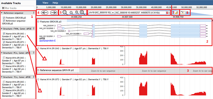
- Available Tracks: Data that is available to be shown in the main viewer is listed in this box. Example in the above figure points to the gene model (2), the reference genome sequence (3), and the reads from 2 donors from the study. The histograms are the number of reads aligned to the reference transcriptome sequence.
- Gene Model: Representation of the gene and its variants, showing exons as boxes and introns as lines.
- Reference Genome: Zooming into a specific exon will eventually reveal the sequence of the reference genome (GRCh38.p2) that the reads were mapped to.
- Scroll Bars: Click on arrows to step along the chromosome.
- Zoom: Click on the magnifying glasses to zoom in or out of the genome. Zooming in will reveal the reference genome sequence at the nucleotide level.
- Chromosome Location: Location of the gene on the chromosome.
- Highlighter: Click this button and then click and drag to high light the data.
- Hide/Show Track Titles: Click on this button to hide or show the track titles that can obscure the data.
Learn about Developing Human Reference Atlases with comprehensive guides and examples from Allen Institute for Brain Science.
Reference Atlases
To complement the RNA-Seq and microarray gene expression data, reference atlases were created at three developmental stages; 15 pcw, 21 pcw and 34 years. The reference atlas are full-color, high-resolution, web-based digital brain atlases accompanied by a systematic, hierarchically organized taxonomy of developing brain structures.
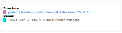
From the heatmap view in the BrainSpan Atlas of the Developing Human Brain, you can see the Structure Ontology list from the selected data point in the heatmap. Clicking on the structure link will bring you to the appropriate developmental stage in the Reference Atlas (adult vs. prenatal).
From the In Situ Hybridization data in the BrainSpan Atlas of the Developing Human Brain, you can also arrive at the Human Brain Atlas Guide by clicking on a hotspot while viewing an experiment in the High Resolution Image Viewer.
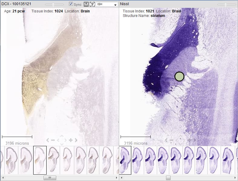
Either of these actions will bring you to the Interactive Atlas Viewer with the structure of interest highlighted in purple.
Clicking on the annotation links from the “Reference Atlas” tab in the banner menu will also take you to the Interactive Atlas Viewers. Supporting data used to create these Atlases is also available for viewing or for download.
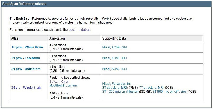
Reference Atlas Viewing Tools
Interactive Atlas Viewer (IAV)
Learn about Brainspan API Developmental Transcriptome with comprehensive guides and examples from Allen Institute for Brain Science.

The BrainSpan Atlas of the Developing Human Brain is a foundational resource for studying transcriptional mechanisms involved in human brain development. The data includes:
- Developmental Transcriptome: RNA sequencing and exon microarray data profiling up to sixteen cortical and subcortical structures across the full course of human brain development
- Prenatal LMD Microarray: High-resolution neuroanatomical transcriptional profiles of ~300 distinct structures spanning the entire brain for four midgestional prenatal specimen
From the API, you can:
Download expression values
Query the correlative and differential search services
Developmental Transcriptome
Experimental Overview and Metadata
The Developmental Transcriptome Study is a broad developmental survey of gene expression in specific brain regions using RNA sequencing and exon microarray techniques. The survey profiles up to sixteen targeted cortical and subcortical structures across the full course of human brain development, spanning pre- and postnatal-development in both males and females.
Each sampling site is associated with a Structure. For convenience, surveyed structures are grouped together in the “Developing Human - Transcriptome” StructureSet.
Typically, for each sample four types of expression values are available:
- RNA-Seq RPKM values summarized to the gene level
- RNA-Seq RPKM values summarized to the exon level
- Normalized exon microarray expression values summarized to the gene level
- Normalized exon microarray expression values summarized to the probeset level
Normalized expression values can be downloaded in several ways:
- From the web application Download page.
- From the “Download this data” link below the heatmap in the web application.
- From the connected data service in the API
All experimental data from this study is associated with the “Developing Human Transcriptome” Product. All gene, exon, probeset, donor and sampling site information can be accessed through the API using RMA queries.
Examples:
- All donors in the Product
http://api.brain-map.org/api/v2/data/Donor/query.xml?include=age&criteria=products[id$eq24]
- All samples in the Product
http://api.brain-map.org/api/v2/data/query.xml?criteria=model::Specimen, rma::criteria,donor(products[id$eq24]), well_known_files(well_known_file_type[name$eqRNASeqSummarizedToGenes]), rma::include,donor(age)
- All prenatal donors in the Product
http://api.brain-map.org/api/v2/data/query.xml?criteria=model::Donor, rma::criteria,products[id$eq24],rma::include,age[embryonic$eqtrue]
- All postnatal donors in the Product
http://api.brain-map.org/api/v2/data/query.xml?criteria=model::Donor, rma::criteria,products[id$eq24],rma::include,age[embryonic$eqfalse]
- All surveyed structures
http://api.brain-map.org/api/v2/data/query.xml?criteria=model::Structure, rma::criteria,structure_sets[name$eq’Developing Human - Transcriptome’], rma::options[only$eq’structures.id,structures.acronym,structures.name,structures.color_hex_triplet’]
Downloading Expression Values
Normalized expression values can be obtained by specifying:
- the required expression type (“set”),
- a list of “probes”,
- a list of donors (optional), and
- a list of structures (optional)
See the connected service page for definitions of service::dev_human_expression parameters.
|Expression Type | “set” parameter | “probe” object|
|— | — | —|
|RNA-Seq RPKM values summarized to the gene level | rna_seq_genes | Gene (ensembl_id not null )|
|RNA-Seq RPKM values summarized to the exon level | rna_seq_exons | GoExons|
|Exon microarray expression values summarized to the gene level | exon_microarray_genes | Gene (entrez_id not null )|
|Exon microarray expression values summarized to the probeset level | exon_microarray_exons | AffymetriProbsets|
RNA-Seq RPKM values summarized to the gene level
Example:
Download RNA-Seq expression values for samples from donor “h376.VI.52” associated with gene CARTPT
- Find Donor ID for “h376.VI.52” (id = 12890)
http://api.brain-map.org/api/v2/data/query.xml?criteria=model::Donor, rma::criteria,[name$eq’H376.VI.52’], rma::options[only$eq’donors.id’]
- Find Gene ID associated with gene CARTPT (id = 1098278)
http://api.brain-map.org/api/v2/data/query.xml?criteria=model::Gene, rma::criteria,[acronym$eq’CARTPT’][type$eq’EnsemblGene’],organism[name$eq’Homo Sapiens’], rma::options[only$eq’genes.id’]
- Use set = rna_seq_genes, Gene (“probe”) and Donor IDs as parameter to the service::dev_human_expression
http://api.brain-map.org/api/v2/data/query.json?criteria=service::dev_human_expression [set$eq’rna_seq_genes’][probes$eq1098278][donors$eq12890]
The output of the service is two top level ordered arrays “probes” and “samples”. For example:
“probes”:[ {“id”:1098278, “name”:“ENSG00000164326”, “gene-id”:9463, “gene-symbol”:“CARTPT”,“gene-name”:“CART prepropeptide”, “entrez-id”:9607,“chromosome”:“5”,“start-position”:“n/a”,“end-position”:“n/a”, “expression_level”:[“5.5566”,“4.9466”,“5.6331”,…]} ], “samples”:[ {“donor”:{“id”:12890,“name”:“H376.VI.52”,“age”:“4 mos”,“color”:“76EB76”}, “structure”:{“id”:10173,“name”:“dorsolateral prefrontal cortex”,“abbreviation”:“DFC”,“color”:“D4B235”}, “top_level_structure”:{“id”:10153,“name”:“neural plate”,“abbreviation”:“NP”,“color”:“D7D8D8”}}, {“donor”:{“id”:12890,“name”:“H376.VI.52”,“age”:“4 mos”,“color”:“76EB76”}, “structure”:{“id”:10185,“name”:“ventrolateral prefrontal cortex”,“abbreviation”:“VFC”,“color”:“C2A335”}, “top_level_structure”:{“id”:10153,“name”:“neural plate”,“abbreviation”:“NP”,“color”:“D7D8D8”}}, {“donor”:{“id”:12890,“name”:“H376.VI.52”,“age”:“4 mos”,“color”:“76EB76”}, “structure”:{“id”:10278,“name”:“anterior (rostral) cingulate (medial prefrontal) cortex”,“abbreviation”:“MFC”,“color”:“E26880”}, “top_level_structure”:{“id”:10153,“name”:“neural plate”,“abbreviation”:“NP”,“color”:“D7D8D8”}}, … ],
Each probe (Gene) contains information about:
- the Ensembl Gene (id, name), and
- the associated NCBI Gene (id, acronym, name, entrez-id), along with
- a vector of normalized expression values in the same order as the “samples” array.
Each sample contains information about:
- the Donor (id, name, age),
- the associated Structure (id, name, acronym and color), and
- the associated top (coarse) level Structure (id, name, acronym and color).
RNA-Seq RPKM values summarized to the exon level
Example:
Download RNA-Seq expression values for samples from donor “h376.VI.52” and all exons associated with gene CARTPT
- Find Donor ID for “h376.VI.52” (id = 12890)
http://api.brain-map.org/api/v2/data/query.xml?criteria=model::Donor, rma::criteria,[name$eq’H376.VI.52’], rma::options[only$eq’donors.id’]
- Find GoExons ID associated with gene CARTPT (id = 279330730,279330740,279330735)
http://api.brain-map.org/api/v2/data/query.xml?criteria=model::GoExon, rma::criteria,gene_association(gene[acronym$eq’CARTPT’]), rma::options[only$eq’go_exons.id’]
- Use set = rna_seq_exons, GoExon (“probe”) and Donor IDs as parameter to the service::dev_human_expression
http://api.brain-map.org/api/v2/data/query.json?criteria=service::dev_human_expression [set$eq’rna_seq_exons’][probes$eq279330730,279330740,2793307356][donors$eq12890]
The output of the service is two top level ordered arrays “probes” and “samples”. For example:
“probes”:[ {“id”:279330730, “name”:“ENSG00000164326”, “gene-id”:1098278, “gene-symbol”:“CARTPT”, “gene-name”:“CART prepropeptide”, “entrez-id”:9607,“chromosome”:“5”,“start-position”:71014989,“end-position”:71015279, “expression_level”:[“5.7282”,“4.8102”,“5.7152”, … ]}, {“id”:279330735, “name”:“ENSG00000164326”, “gene-id”:1098278,“gene-symbol”:“CARTPT”, “gene-name”:“CART prepropeptide”, “entrez-id”:9607,“chromosome”:“5”,“start-position”:71015405,“end-position”:71015790, “expression_level”:[“4.4128”,“3.8230”,“4.3135”, … ]}, {“id”:279330740, “name”:“ENSG00000164326”, “gene-id”:1098278,“gene-symbol”:“CARTPT”, “gene-name”:“CART prepropeptide”, “entrez-id”:9607,“chromosome”:“5”,“start-position”:71016334,“end-position”:71016875, “expression_level”:[“5.9593”,“5.4664”,“6.1137”, … ]} ], “samples”:[ {“donor”:{“id”:12890,“name”:“H376.VI.52”,“age”:“4 mos”,“color”:“76EB76”}, “structure”:{“id”:10173,“name”:“dorsolateral prefrontal cortex”,“abbreviation”:“DFC”,“color”:“D4B235”}, “top_level_structure”:{“id”:10153,“name”:“neural plate”,“abbreviation”:“NP”,“color”:“D7D8D8”}}, {“donor”:{“id”:12890,“name”:“H376.VI.52”,“age”:“4 mos”,“color”:“76EB76”}, “structure”:{“id”:10185,“name”:“ventrolateral prefrontal cortex”,“abbreviation”:“VFC”,“color”:“C2A335”}, “top_level_structure”:{“id”:10153,“name”:“neural plate”,“abbreviation”:“NP”,“color”:“D7D8D8”}}, {“donor”:{“id”:12890,“name”:“H376.VI.52”,“age”:“4 mos”,“color”:“76EB76”}, “structure”:{“id”:10278,“name”:“anterior (rostral) cingulate (medial prefrontal) cortex”,“abbreviation”:“MFC”,“color”:“E26880”}, “top_level_structure”:{“id”:10153,“name”:“neural plate”,“abbreviation”:“NP”,“color”:“D7D8D8”}}, … ],
Each probe (GoExon) contains information about:
- the GoExon (id, name), and
- the associated Ensembl Gene (id, acronym, name, entrez-id), along with
- a vector of normalized expression values in the same order as the “samples” array.
Each sample contains information about:
- the Donor (id, name, age),
- the associated Structure (id, name, acronym and color), and
- the associated top (coarse) level Structure (id, name, acronym and color).
Normalized exon microarray expression values summarized to the gene level
Example:
Download exon microarray expression values for samples from donor “h376.VI.50” associated with gene CARTPT
- Find Donor ID for “h376.VI.50” (id = 12296)
http://api.brain-map.org/api/v2/data/query.xml?criteria=model::Donor, rma::criteria,[name$eq’H376.VI.50’], rma::options[only$eq’donors.id’]
- Find Gene ID associated with gene CARTPT (id = 9463)
http://api.brain-map.org/api/v2/data/query.xml?criteria=model::Gene, rma::criteria,[acronym$eq’CARTPT’][type$eq’NcbiGene’],organism[name$eq’Homo Sapiens’], rma::options[only$eq’genes.id’]
- Use set = exon_microarray_genes, Gene (“probe”) and Donor IDs as parameter to the service::dev_human_expression
http://api.brain-map.org/api/v2/data/query.json?criteria=service::dev_human_expression [set$eq’exon_microarray_genes’][probes$eq9463][donors$eq12296]
The output of the service is two top level ordered arrays “probes” and “samples”. For example:
“probes”:[ {“id”:9463, “name”:“ENSG00000164326”, “gene-id”:9463, “gene-symbol”:“CARTPT”, “gene-name”:“CART prepropeptide”, “entrez-id”:9607,“chromosome”:“5”,“start-position”:“n/a”,“end-position”:“n/a”, “expression_level”:[“8.1073”,“5.9564”,“6.3102”,“7.0532”,“9.6157”,“7.1290”,“5.1168”,“4.4212”,“4.2779”], “z-score”:[“1.3547”,“0.0538”,“0.2678”,“0.7172”,“2.2670”,“0.7630”,“-0.4541”,“-0.8748”,“-0.9615”]} ], “samples”:[ {“donor”:{“id”:12296,“name”:“H376.VI.50”,“age”:“4 mos”,“color”:“80FF80”}, “structure”:{“id”:10278,“name”:“anterior (rostral) cingulate (medial prefrontal) cortex”,“abbreviation”:“MFC”,“color”:“E26880”}, “top_level_structure”:{“id”:10153,“name”:“neural plate”,“abbreviation”:“NP”,“color”:“D7D8D8”}}, {“donor”:{“id”:12296,“name”:“H376.VI.50”,“age”:“4 mos”,“color”:“80FF80”}, “structure”:{“id”:10243,“name”:“posterior (caudal) superior temporal cortex (area 22c)”,“abbreviation”:“STC”,“color”:“D670A0”}, “top_level_structure”:{“id”:10153,“name”:“neural plate”,“abbreviation”:“NP”,“color”:“D7D8D8”}}, … ]
Each probe (Gene) contains information about:
- the NCBI Gene (id), and
- the associated NCBI Gene (id, acronym, name, entrez-id), along with
- a vector of normalized expression values in the same order as the “samples” array, and
- a vector of z-score values in the same order as the “samples” array. Note: z-score is computed independently over all samples for each gene.
Each sample contains information about:
- the Donor (id, name, age),
- the associated Structure (id, name, acronym and color), and
- the associated top (coarse) level Structure (id, name, acronym and color).
Normalized exon microarray expression values summarized to a probeset level
Download exon microarray expression values for samples from donor “h376.VI.50” for all probesets associated with gene CARTPT
- Find Donor ID for “h376.VI.50” (id = 12296)
http://api.brain-map.org/api/v2/data/query.xml?criteria=model::Donor, rma::criteria,[name$eq’H376.VI.50’], rma::options[only$eq’donors.id’]
- Find AffymetrixProbeset ID associated with gene CARTPT (id = 280550735,280550750,280550740,280550730,280550745)
http://api.brain-map.org/api/v2/data/query.xml?criteria=model::AffymetrixProbeset, rma::criteria,gene_association(gene[acronym$eq’CARTPT’](organism[name$eq’Homo Sapiens’])), rma::options[only$eq’affymetrix_probesets.id’]
- Use set = exon_microarray_exons, AffymetrixProbeset (“probe”) and Donor IDs as parameter to the service::dev_human_expression
http://api.brain-map.org/api/v2/data/query.json?criteria=service::dev_human_expression [set$eq’exon_microarray_exons’][probes$eq280550735,280550750,280550740,280550730,280550745][donors$eq12296]
The output of the service is two top level ordered arrays “probes” and “samples”. For example:
“probes”:[ {“id”:280550735, “name”:“ENSG00000164326”, “gene-id”:9463, “gene-symbol”:“CARTPT”, “gene-name”:“CART prepropeptide”, “entrez-id”:9607,“chromosome”:“5”,“start-position”:71015125,“end-position”:71015265, “expression_level”:[“8.1073”,“6.4681”,“6.3102”,“7.0532”,“9.4350”,“7.1290”,“5.1560”,“5.0550”,“4.9879”], “z-score”:[“1.4783”,“0.0367”,“-0.1021”,“0.5513”,“2.6458”,“0.6179”,“-1.1171”,“-1.2059”,“-1.2649”]}, {“id”:280550750, “name”:“ENSG00000164326”, “gene-id”:9463, “gene-symbol”:“CARTPT”, “gene-name”:“CART prepropeptide”, “entrez-id”:9607,“chromosome”:“5”,“start-position”:71016613,“end-position”:71016799, “expression_level”:[“10.1951”,“8.8021”,“7.7846”,“9.4317”,“11.8110”,“10.0210”,“6.1850”,“5.6075”,“4.5526”], “z-score”:[“1.2342”,“0.6566”,“0.2348”,“0.9177”,“1.9041”,“1.1620”,“-0.4284”,“-0.6678”,“-1.1052”]}, ], “samples”:[ {“donor”:{“id”:12296,“name”:“H376.VI.50”,“age”:“4 mos”,“color”:“80FF80”}, “structure”:{“id”:10278,“name”:“anterior (rostral) cingulate (medial prefrontal) cortex”,“abbreviation”:“MFC”,“color”:“E26880”}, “top_level_structure”:{“id”:10153,“name”:“neural plate”,“abbreviation”:“NP”,“color”:“D7D8D8”}}, {“donor”:{“id”:12296,“name”:“H376.VI.50”,“age”:“4 mos”,“color”:“80FF80”}, “structure”:{“id”:10243,“name”:“posterior (caudal) superior temporal cortex (area 22c)”,“abbreviation”:“STC”,“color”:“D670A0”}, “top_level_structure”:{“id”:10153,“name”:“neural plate”,“abbreviation”:“NP”,“color”:“D7D8D8”}}, … ]
Each probe (Gene) contains information about:
- the AffymetrixProbeset (id), and
- the associated NCBI Gene (id, acronym, name, entrez-id), along with
- a vector of normalized expression values in the same order as the “samples” array, and
- a vector of z-score values in the same order as the “samples” array. Note: z-score is computed independently over all samples for each gene.
Each sample contains information about:
- the Donor (id, name, age),
- the associated Structure (id, name, acronym and color), and
- the associated top (coarse) level Structure (id, name, acronym and color).
Differential Search
Differential search find “probes” that show the greatest difference in expression values between two sets (target and contrast) of user-defined structures. For each probe, a 2-sample t-test is performed followed by Benjamini and Hochberg false discovery rate correction. The null hypothesis is that the average expression level of samples in the contrast set of structures is greater than or equal to the average expression level of samples in the target set of structures. A statistically significant result (p-value less than user-defined threshold) allows us to reject the null hypothesis and conclude that the average expression level of samples in the target set of structures is greater than the average expression level of samples in the contrast set of structures. Resulting p-values are sorted in ascending order. Search results can also be sorted by fold-change (log ratio of expression) in descending order.
The differential search function can be accessed through the Web application or using the API.
See the connected service page for definitions of service::dev_human_differential parameters.
Example:
Differential search for genes with higher expression in “striatum” than in the whole “neural plate” over all donors for each of the four types of expression data.
- Find Structure ID for “striatum” (id = 10333 )
http://api.brain-map.org/api/v2/data/query.xml?criteria=model::Structure, rma::criteria,[name$il’striatum’],ontology[name$eq’Developing Human Brain Atlas’], rma::options[only$eq’structures.id’]
- Find Structure ID for “neural plate” (id = 10153)
http://api.brain-map.org/api/v2/data/query.xml?criteria=model::Structure, rma::criteria,[name$il’neural plate’],ontology[name$eq’Developing Human Brain Atlas’], rma::options[only$eq’structures.id’]
- Differential search for gene-level RNA-Seq data (set = rna_seq_genes)
http://api.brain-map.org/api/v2/data/query.xml?criteria=service::dev_human_differential [set$eq’rna_seq_genes’][structures1$eq10153][structures2$eq10333][sort_by$eq’fold-change’]
- Differential search for exon-level RNA-Seq data (set = rna_seq_exons )
http://api.brain-map.org/api/v2/data/query.xml?criteria=service::dev_human_differential [set$eq’rna_seq_exons’][structures1$eq10153][structures2$eq10333][sort_by$eq’fold-change’]
- Differential search for gene-level exon microarray data (set = exon_microarray_genes )
http://api.brain-map.org/api/v2/data/query.xml?criteria=service::dev_human_differential [set$eq’exon_microarray_genes’][structures1$eq10153][structures2$eq10333][sort_by$eq’fold-change’]
- Differential search for probeset-level exon microarray data (set = exon_microarray_exons )
http://api.brain-map.org/api/v2/data/query.xml?criteria=service::dev_human_differential [set$eq’exon_microarray_exons’][structures1$eq10153][structures2$eq10333][sort_by$eq’fold-change’]
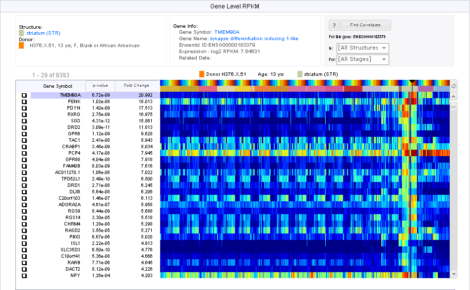
Example:
Differential search for genes with higher expression at 8-9 pcw than at 10-12 pcw over the whole “neural plate” for each of the four types of expression data.
- Find Structure ID for “neural plate” (id = 10153)
http://api.brain-map.org/api/v2/data/query.xml?criteria=model::Structure, rma::criteria,[name$il’neural plate’],ontology[name$eq’Developing Human Brain Atlas’], rma::options[only$eq’structures.id’]
- Find Donor IDs for donors within age 8-9 pcw (id = 12833,13058)
http://api.brain-map.org/api/v2/data/query.xml?criteria=model::Donor, rma::criteria,products[name$eq’Developing Human Transcriptome’],age[embryonic$eqtrue][days$ge56][days$le63], rma::options[only$eq’donors.id’]
- Find Donor IDs for donors within age 10-12 pcw (id = 12835,12960,13060)
http://api.brain-map.org/api/v2/data/query.xml?criteria=model::Donor, rma::criteria,products[name$eq’Developing Human Transcriptome’],age[embryonic$eqtrue][days$ge70][days$le84], rma::options[only$eq’donors.id’]
- Differential search for gene-level RNA-Seq data (set = rna_seq_genes)
http://api.brain-map.org/api/v2/data/query.xml?criteria=service::dev_human_differential [set$eq’rna_seq_genes’][donors1$eq12835,12960,13060][donors2$eq12833,13058] [structures1$eq10153][structures2$eq10153][sort_by$eq’fold-change’]
- Differential search for exon-level RNA-Seq data (set = rna_seq_exons )
http://api.brain-map.org/api/v2/data/query.xml?criteria=service::dev_human_differential [set$eq’rna_seq_exons’][donors1$eq12835,12960,13060][donors2$eq12833,13058] [structures1$eq10153][structures2$eq10153][sort_by$eq’fold-change’]
- Differential search for gene-level exon microarray data (set = exon_microarray_genes )
http://api.brain-map.org/api/v2/data/query.xml?criteria=service::dev_human_differential [set$eq’exon_microarray_genes’][donors1$eq12835,12960,13060][donors2$eq12833,13058] [structures1$eq10153][structures2$eq10153][sort_by$eq’fold-change’]
- Differential search for probeset-level exon microarray data (set = exon_microarray_exons )
http://api.brain-map.org/api/v2/data/query.xml?criteria=service::dev_human_differential [set$eq’exon_microarray_exons’][donors1$eq12835,12960,13060][donors2$eq12833,13058] [structures1$eq10153][structures2$eq10153][sort_by$eq’fold-change’]
Correlative Search
Correlative search finds “probes” with expression profile similar that of a to a selected seed “probe” over all samples within a user-specified structure and for user-specified donors. Pearson’s correlation coefficient is computed for all probes and the results ranked in descending order.
The correlative search function can be accessed through the Web application or using the API.
See the connected service page for definitions of service::dev_human_correlation parameters.
Example:
Correlative search for “probes” with similar expression to PVALB over the whole brain
- Correlative search for gene-level RNA-Seq data ( seed ?Ensembl Gene id = 1089164, set = rna_seq_genes )
http://api.brain-map.org/api/v2/data/query.xml?criteria= service::dev_human_correlation[set$eqrna_seq_genes][probes$eq1089164][structures$eq10153]
- Correlative search for exon-level RNA-Seq data ( seed GoExon id = 278724739, set = rna_seq_exons )
http://api.brain-map.org/api/v2/data/query.xml?criteria= service::dev_human_correlation[set$eqrna_seq_exons][probes$eq278724739][structures$eq10153]
- Correlative search for gene-level exon microarray data (seed NCBI Gene id = 5784, set = exon_microarray_genes )
http://api.brain-map.org/api/v2/data/query.xml?criteria= service::dev_human_correlation[set$eqexon_microarray_genes][probes$eq5784][structures$eq10153]
- Correlative search for probeset-level exon microarray data ( seed AffymetrixProbeset id = 281337753, set = exon_microarray_exons )
http://api.brain-map.org/api/v2/data/query.xml?criteria= service::dev_human_correlation[set$eqexon_microarray_exons][probes$eq281337753][structures$eq10153]
Learn about Brainspan Prenatal LMD Microarray with comprehensive guides and examples from Allen Institute for Brain Science.
Searching The Prenatal Laser Microdissection (LMD) Microarray Data
Three search types are available: (1) Gene Search, to obtain gene expression data for specific genes of interest, (2) Differential Search, to compare expression between two sets of brains structures, and (3) Correlative Search, to find genes that have an expression pattern similar to a “seed gene” selected from the results of a Gene or a Differential search.
Clicking on the “?” button from any search type will take you to the appropriate help section.
Gene Search
To search for probes associated with a specific gene, select the Gene Search radio button, type the gene name, gene symbol, Entrez Gene ID or probe name in the search box and click the “Search” button. Alternatively, select a category from the tag cloud. The font size of the words in the cloud correspond to the number of genes linked to each category. Genes were linked to each category using online tools such as the PANTHER.
To restrict the set of probes displayed, check the boxes next to the Gene Symbols and click the View Selection Heatmap button at the bottom of the page (see heat map figure below).
Differential Search
Another common usage of gene expression databases is to find genes that show enrichment of expression in one region compared to another region. This type of query is supported by the Differential Search mode. Select the “Differential Search” radio button. To find genes or probes with an enhanced gene expression profile in one or more structures when compared to one or more other structures, enter the target brain structure in the top search box and your contrast regions in the bottom search box. You also have the option to filter your search by donor. Once you have made your selections, click on the Search button.
To enter the structures, you can simply type the acronyms (separated by semi-colons) in the search boxes, or select them from the drop down ontology viewer.
Your search will return genes exhibiting higher expression in the target domain compared to the contrast domain. You can filter the displayed data on the heatmap by clicking the “Filter Heatmap” function below the heatmap. A menu will open allowing you to select both the structures and the developmental stages. Search results are sorted either by p-value or fold change, indicated by the arrow on the buttons over the column of genes. To alter the sort parameter, click on either the “p value” or the “fold-change” buttons.
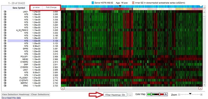
To perform the previous search in reverse, click the toggle button to the left of the Search button.
Correlative Search
In using gene expression databases, a “search by example” feature is also highly desirable as genes with similar expression patterns may be related in function. The Find Correlates search utility will accomplish this function. This search by example facility is also available in the Allen Human Brain Atlas, and in the Allen Mouse Brain Atlas and the Allen Developing Mouse Brain Atlas as the NeuroBlast function.
Once you have identified a gene of interest, to find other genes with spatial expression profiles similar to your gene of interest, first select your probe by clicking on any cell in the heat map related to that probe. You will see that probe listed in the box above the right hand side of the heat map. Then select the brain structure(s) and donor(s) in which you would like to see a similar expression pattern, and click “Find Correlates”. This action will return probes with a similar expression profile in the brain region(s) and donor(s) in which you are interested.
Only regions selected for the search will be displayed. To see the search results across the entire brain, turn off the “Restrict Domains” function at the bottom of the heat map. You can see “anti-correlated” genes by toggling the sort order on column “r” or scrolling to the bottom of the heat map.
Gene Classification
When you are viewing heatmap data, there will be a “Gene Classification” radio button available. When the gene classification radio button is selected, you can search for enhanced gene expression from one of the categories in the drop down menu.
Data Visualization
The visualization page for the prenatal LMD microarray data is divided into two sections:
- The bottom section contains the heatmap representation of the data returned by a search operation.
- The top section contains probe, sample and expression information for a data point selected by clicking a location in the heat map.
Heatmaps
Based on your search, the resulting microarray data sets are presented as a matrix with brain structure and donor on the horizontal x-axis and gene probes on the vertical y-axis. On the horizontal axis, donors are represented in the first row and by the three distinct blue colors. The next row represents brain structures and are organized in ontological order. To toggle between sorting initially by structure or by donor, click the toggle button (see below). On the vertical axis, each row represents a probe rather than a gene, since multiple probes were used to measure gene expression for a gene.

The microarray data is presented in a heat map format where the colors of the heat map correspond either to raw data or to a normalized (z-score) expression level of a probe. Default heat map colors are in the green - red scale, where green represents low expression values and red, high expression values. The window and level for the colors may be adjusted, and other color schemes may be selected by using the Color Map control under the heat map.
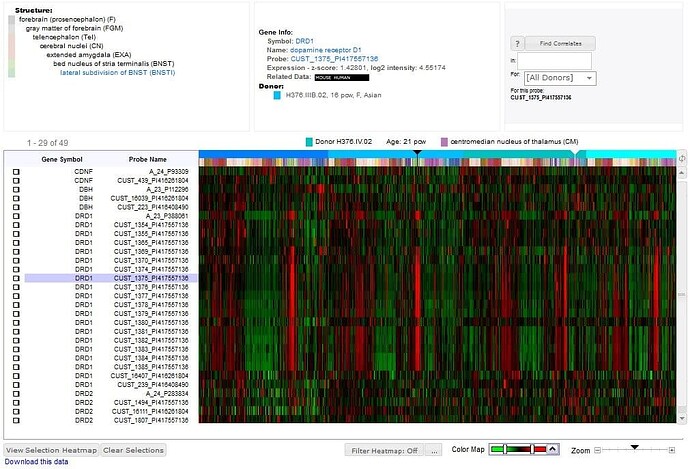
You can select a set of probes for later use by selecting the check-boxes beside the list of gene symbols. Your choices are stored in a browser cookie in your computer and will remain in effect until you click the “Clear Selections” button or clear your Web browser’s cookie cache. Click the “View Selections” button to see your selections.
Detailed Information Section
Clicking on a cell of the heat map populates the top section of the page with detailed information about the selected cell. This information includes our structure ontology which when you click the blue link at the bottom will take you to the Reference Atlas. It also includes Gene Information; gene symbol, gene name, probe name (when the gene or probe links are clicked you will be taken to a Gene Details page), expression values (log2 intensity and z-score), and the donor details.
The section also contains buttons to navigate to related data in other Allen Brain Atlas resources, as well as links to external pages with additional data on the specific gene and probe.

Gene Details
Clicking on the Gene Symbol or Gene Name takes you to the gene details page.
The gene details page displays information about the gene in three parts. The first lists metadata specifically about the gene, including Gene Name, Aliases, Organism, related data from other Allen Brain Atlas resources, Entrez gene ID and Chromosome.
The second part outlines information specific for the probe originally selected from the heatmap, including Probe Name, NCBI Accession Number, Probe length, Sequence Data, probe type, transcript GI identifier and GC percentage.
The third part of the gene detail page is a visual representation of gene expression throughout the brain. The first row of images includes seven representative sections from the Reference Atlas with each structure color coded as in the original heatmap. The next row of four images illustrates gene expression in a select section from each of the donors.
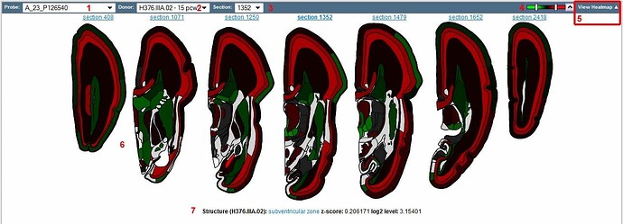
Navigating this structural representation of gene expression:
- Probe: The dropdown menu allows you to navigate to other probes for this particular gene.
- Donor: The dropdown menu allows you to navigate to other donors.
- Section: Indicates which of the seven sections is portrayed in the second row of images. The dropdown menu allows you to choose which representative section is portrayed over the four different donors.
- Color Map Bar: Displays different normalized (z-score) color representations of the heat map data (i.e. blue-red vs. green-red) or log2 normalized expression where the color scale ranges from dark blue, representing low expression, and passes through cyan, yellow, orange and finally to dark red, representing high expression. Clicking on the arrow will allow you to change the color map.
- View Heatmap: Clicking on “View Heatmap” will take you back to the microarray heatmap data.
- Atlas Sections: Seven sections from the reference atlas representing gene expression in each structure. Clicking on the link above one of the sections will select that section to be displayed in the second row if images. Hovering over a section with your mouse will bring up the ontology below the sections and indicate the name of the region/structure. Clicking on an image will highlight that structure in all of the sections that include that structure. When a structure is selected in this fashion, hovering your mouse over another structure will bring up the name and gene expression of that structure for comparison.
- Ontology: The name of the structure and gene expression values of that structure for the probe and donor selected. Clicking on the link will take you to the Reference Atlas
The second row of images shows a representative section from each of the donors to allow for comparison of gene expression values between donors.

Learn about Specimens Of The Aging Dementia And TBI Project with comprehensive guides and examples from Allen Institute for Brain Science.
The Adult Changes in Thought (ACT) study is a longitudinal population-based prospective cohort study of brain aging and incident dementia in the Seattle metropolitan area. This cohort includes 5,000+ participants of which more than 700 have agreed to autopsy upon their death. From this smaller population who agreed to an autopsy, participants who had experienced at least one mild to moderate traumatic brain injury (TBI) with a loss of consciousness were chosen for this study, along with sex-, age- and post mortem interval- (PMI) matched controls. The specimens page lists this cohort sub-group in a sortable matrix, which allows for exploration of the donors by various demographic and/or pathological features.
Clicking on the column header will sort alphanumerically, clicking twice will toggle between ascending and descending order.
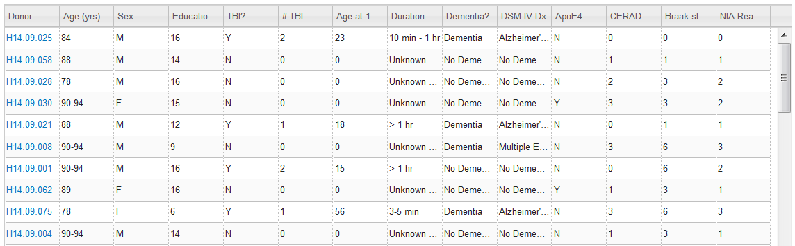
Specimen Detail Page
Clicking on a link from the Specimens page or clicking on a circle from the t-SNE plot from one of the data snapshots will open a specimen detail page. This page allows access to the data collected from this donor including Gene Detail, Gene Set, Neuropathology Metric Detail, Neuropathology Metrics, Donor Detail and Image Data.
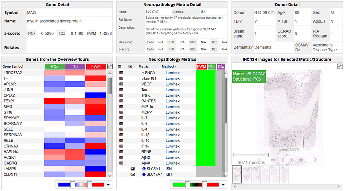
Gene Detail
Once a data point is selected in the gene set panel, details of that gene will populate this space including the gene symbol, the gene name, the expression value from the RNA-Sequencing data, and a link to other Allen Institute datasets that have measured this gene.
Gene Set
The gene set panel is populated by the genes in the data snapshot (if you linked from a specific snapshot) or by the entire gene set that was used in all the snapshots (if you arrived from the Specimens page). The column headers are the samples from this donor that were sequenced. The gene set is a smaller version of the heatmap from the RNA-Sequencing data limited by the number of genes and the the donor. The icon in the top right-hand corner of the gene set display will link you to the RNA-Seq data for all donors and samples.
Neuropathology Metric Detail
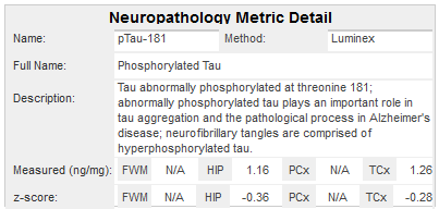
Once a datapoint in the neuropathology metrics display is selected, metric detail will populate this panel (and if the metrics came from an image, the image will also populate the image data panel) including the short and long names of the metric, the method used to collect the metric, a description of what the metric is and it’s significance, and the values collected or calculated.
Neuropathology Metrics
This panel lists all the neuropathology assays collected on this donor. To populate data from this panel into the neuropathology metric detail panel, click on a data point in the heatmap.
| Column | Description |
|---|---|
 | An icon in this column indicates there is a value for this metric. Clicking on the column header will sort the data by this column. |
 | An icon in this column indicates there is image data for this metric. Clicking on the column header will sort the data by this column. |
| Metric | Lists the assay that was measured/calculated. Also listed in the neuropathology metric detail display. |
| Method | Lists the method that was to acquire the metric. Also listed in the neuropathology metric detail display. |
| Heatmap Columns | Brain regions from which the metric was collected/calculated. This data is presented in heatmap form, and the color range can be adjusted by using the sliders on the color map below the heatmap. |
Donor Detail
The donor detail panel is populated with metadata from this donor including Donor ID, Age, Sex, Reported TBI, tbi, Presence of ApoE4 allele, Braak stage, CERAD score, NIA Reagan, Dementia diagnosis and DSM-IV diagnosis.
Image Data
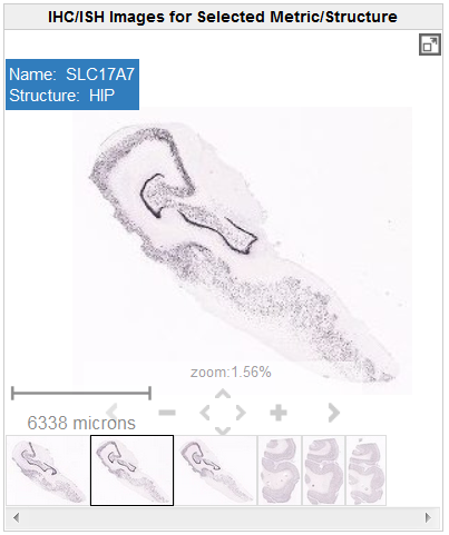
The image data panel is populated once a data point has been selected in the neuropathology metrics panel. This image viewer includes a main viewer, thumbnail views of all the images in the series - which when selected will bring up the image in the main viewer, the name of the assay and the location in the top left-hand corner of the viewer and on-screen navigation tools. Zoom in and out with the onscreen tools or use the keyboard commands.
In the top right hand corner of the viewer is an icon that will take you to a High Resolution Image Viewer.
High Resolution Image Viewer
Once you click on the full screen viewer button, you will be taken to a screen with side by side viewers (when available). The left hand viewer shows the image series you launched the viewer from and the right hand viewer displays the closest reference image from the same specimen block. This viewer is very similar to the viewer on the donor page with more functionality (see the toolbar features).
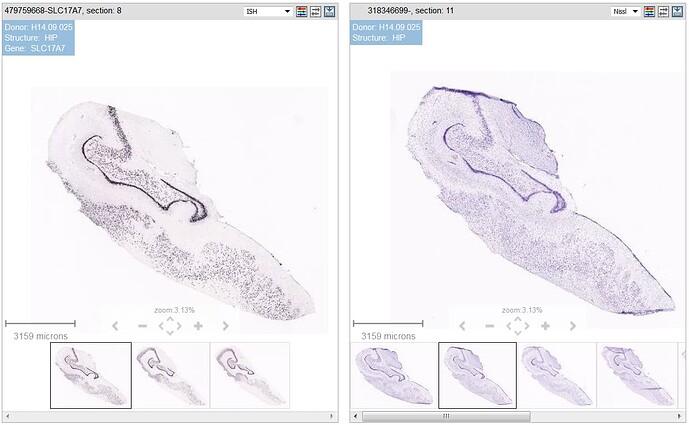
Toolbar
| Icon | Description |
|---|---|
 | Toggle between the current image, other reference images or the expression view |
 | Click to open adjustable image filters |
 | Find nearest reference image in the adjacent viewer |
 | Download the current image |
Scale Bar
Shows the current viewing resolution of the image, in microns. This value dynamically changes as you zoom in/out of the image. You can position the scale bar anywhere on the main image by dragging the scale bar by its ruler.
You can toggle the orientation of the scale bar from horizontal to vertical by clicking on the scale bar text. When you download an image, the scale bar is not included with the image.
Keyboard Commands
Expression Mask Colors
The Expression Mask image display highlights those cells that have the highest probability of gene expression using a heat map color scale (from low/blue to high/red).
Learn about Human Brain Atlas In Situ Hybridization ISH Data with comprehensive guides and examples from Allen Institute for Brain Science.
Gene expression data is available as colorimetric in situ hybridization (ISH) images for specific brain regions. Images are grouped into image series that comprise an experiment. An experiment consists of a sequence of slides from the same specimen and that receive the same treatment, whether it is Nissl staining or ISH with a probe for a particular gene.
ISH data is available for five distinct studies: The Cortex Study (1,000 Gene Survey in Cortex), Schizophrenia Study, Autism Study, Subcortex Study and Neurotransmitter Study. Please refer to the In situ hybridization white paper in the Allen Human Brain Atlas Documentation tab for details.
Choose among the following options for retrieving the data:
Searching
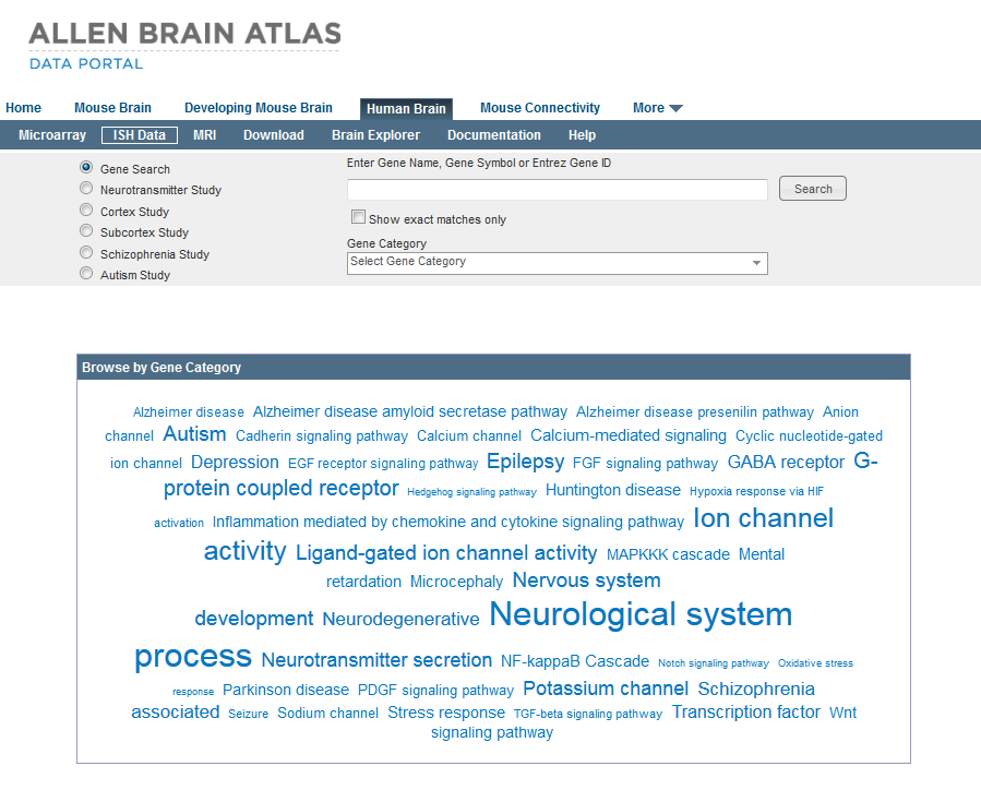
You can search for enhanced gene expression in various categories by selecting on a category from the tag cloud or by selecting multiple categories from the Gene Category drop down menu. The font size in the tag cloud is proportional to the number of genes associated with that category. The categories were created by online search engines such as PANTHER.
Gene Search
You can search for experiments associated with a gene using its gene symbol, name, or Entrez Gene ID. First, select the “Gene” radio button, type the search term in the input box and click the “Search” button. You will be offered suggestions to choose from while you type, but you can also search by typing the first three or more letters in a gene name or symbol and appending an asterisk ( * ) as a wildcard.
Search by Study
Data includes ISH experiments from five separate projects including: Neurotransmitter Study, 1,000 Gene Survey in Cortex (Cortex Study), Subcortex study, Schizophrenia Study and Autism Study. Please refer to the In situ hybridization white paper and the gene list under the Allen Human Brain Atlas Documentation page for details. A brief description of the study methods are included on the landing page for each study.
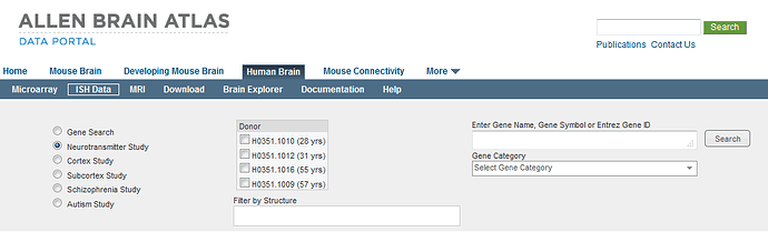

You can restrict your search to a single study by selecting the relevant radio button: Neurotransmitter Study, Cortex Study, Subcortex Study, Schizophrenia Study or Autism Study. You will then have a choice to limit your search based on additional criteria such as sex of the donor, hemisphere, etc., depending on the study. Once a radio button for a specific study is selected, you will have the choice to select experiments based on one or more gene categories from the drop-down menu. While in the Subcortex or Neurotransmitter Study (by selecting the appropriate radio button), you also have the option to filter your gene search by structure.
Type a search term in the input box and click the “Search” button. Clicking the “Search” button without an entry in the input box will return the complete list of genes and the accompanying data for that study.
The following search criteria can be specified in the text box to the right of the categories. If you copy and paste in a list of terms delimited by tabs or carriage returns they will automatically be converted into a list of search criteria separated by the OR operator ( | ).
- Gene symbol
- Gene name
- Entrez gene ID
- Homologene Group ID
- NCBI accession number
- Probe name
Boolean Syntax
The following special operators can be used to build queries:
- AND, OR and NOT may be used in place of their corresponding operators. They must be upper case.
- The AND operator (&) is implicit, so spaces between words that are not separated by an operator will be treated like an &.
- OR (|) has higher operator precedence than AND (&).
- Parenthesis can be used to group criteria, but nested parenthesis are not supported at this time.
- The NOT operator (!) is not supported within parenthesis.
Gene Classification
At any time during your visit to this website, you can search on the categories in the tag cloud by selecting the “Gene Classification” radio button and then selecting a category from the drop down menu.
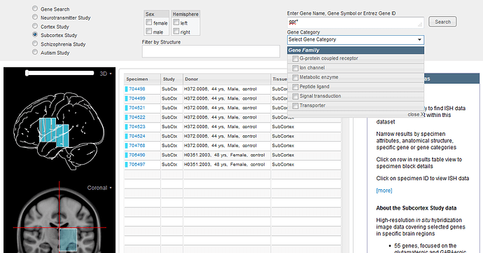
Gene Search Returns
Your search will return a list of specimen blocks which include experiments that fit your search criteria, and an interactive visual display to provide structural context of where the specimen was sampled from. Use the slider bar to rotate the top image, and the drop-down menu to view either coronal or sagittal planes in the lower image. You can filter the search results by clicking on one or more blocks from the visual display. To select more than one block, press Shift and click on the block. Click on the blocks a second time to deselect them or click on the “Clear Selections” button below the display.
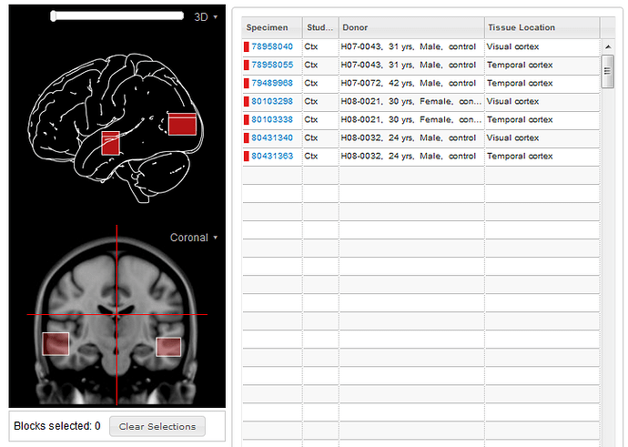
The list of experimental returns includes:
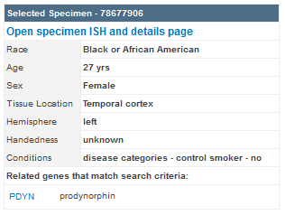
Clicking on the donor will open a panel on the right with more metadata regarding your specimen.
This panel includes demographic information of the donor including their race, gender, age, the tissue location, handedness and any relevant conditions. If your search was not gene specific, all genes that were assayed on this specimen block will be listed under “Related genes that match search criteria:”. You can open the Specimen Detail Information page by clicking the link labeled “Open specimen ISH and details page” or you can directly view the experimental detail by clicking on the gene abbreviation.
Viewing Images
Experiment Details Page
Clicking on the Experiment ID from the search results page will take you to an experimental details page which includes metadata on the experiment, the specimen and the probe as well as related institute data links and a ZAP viewer for all images in the series.
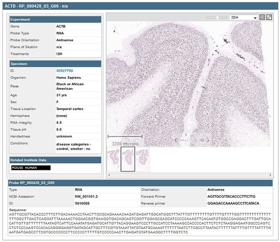
This data can be downloaded as an XML file by clicking the link in “This data is also available as XML”.
Zoom and Pan (ZAP) Image Viewer

The gene symbol or treatment type is displayed in the title bar along with the image series ID. Additional details are displayed across the top of the viewing area, including but not limited to the tissue index and tissue location.
Thumbnails for the entire image series are displayed across the bottom of the viewer in section order. Click a thumbnail to select it for viewing, or use the keyboard to navigate through the set. The current selection is outlined in black.
Scale Bar
Shows the current viewing resolution of the image, in microns. This value dynamically changes as you zoom in/out of the image. You can position the scale bar anywhere on the main image by dragging the scale bar by its ruler.

You can toggle the orientation of the scale bar from horizontal to vertical by clicking on the scale bar text.
Toolbar
| Icon | Description |
|---|---|
 | Adjust contrast on the main image |
 | Select ISH, Nissl, or Expression image type |
 | View image series in contact sheet form |
 | Show current image in a High Resolution Image Viewer |
 | Open a new window to view the image series’ details |
 | Close the current image viewer |
Keyboard Commands
Expression Mask Colors
The Expression mask image display highlights those cells that have the highest probability of gene expression using a heat map color scale (from low/blue to high/red).
High Resolution Image Viewer
Side-by-Side Nissl Viewing
Once you click on the full screen viewer button, you will be taken to a screen with side-by-side viewers. The left hand viewer shows the ISH image series and the right hand viewer displays the Nissl image series from the same specimen block. By default, the nearest Nissl section to the ISH image you are interested in will be shown and synched with the section you are viewing. Click the “Sync” checkbox to manually correct any synching between the images. Clicking on another ISH image will automatically display its nearest Nissl section. Clicking on an image thumbnail in the Nissl image series will automatically take you to the nearest ISH image. While the “Sync” box is checked the Pan and Zoom functions will affect both ISH and Nissl images.

Colored circles in the Nissl slides are hotspots - regions that when moused over list the brain regions manually labeled by our Annotation team. Clicking on one of the hotspots will take you to the Interactive Atlas Viewer, which will provide a spatial context for the structure you have indicated inside our Human Brain Atlas Guide.
To download an image, click on the Download icon (see below).

Specimen Detail Information
Clicking on the specimen link from the search results page or on the specimen link in the experiment details page will take you to detailed specimen information. Specimen detail information includes:
- Specimen Information
- Spatial Context
- Section Information
- Gene Information
- Image Viewer
- Nearest Nissl Image
- Select experiments for the Multiple Experiment Viewer
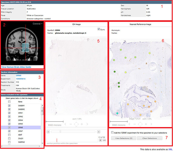
Donor/Specimen Metadata

Specimen ID - internal ID
Age - years
Sex - male or female
Tissue Location - tissue origination in brain
Hemisphere - right or left hemisphere tissue origination
RNA Integrity Number - metric indicating RNA integrity from tissue. Ranges from 1 to 10 (degraded to intact RNA)
pH - tissue sample pH
Race - ethnicity
Handedness - right, left, or ambidextrous
Conditions - disease conditions, smoker
Spatial Context
Specimen blocks are drawn onto an MRI image of the donor brain in either the coronal or saggital plane. Click the drop-down menu in the top right-hand corner of the MRI to change orientation.
To view the Human Brain Atlas Guide, click on the link below the image to open an Interactive Atlas Viewer in a new window.
Section Information
The section information box lists information from the current gene pictured in the image viewer including the gene name, the experiment ID, the section number, the treatment and which study the data came from.
Gene Information
The Gene information section lists the genes that were assayed in this specimen block.
All genes from this specimen block are listed, but only ones selected in your original search criteria are selected. You can select fewer more or less genes/histological stains to view in the image viewer by selecting the checkboxes next to the gene/stain(s) you would like to view.
Image Viewer
The viewer displays the image from the current gene highlighted in the gene information box. Below the image is an indicator of the position in the specimen block of that particular section, as well as a visualization of the depth of the section into the block. You can view the sections in order (default or by clicking the 123 button (see below) or grouped by gene button (see below).


You can navigate these images similar to the ZAP Image Viewer; with the on-screen navigation tools or the Keyboard Commands.
Nearest Nissl Image
When the “Sync” box is checked in the Image Viewer, the closest reference section will be automatically loaded in this viewer. As you are browsing images in the Image Viewer, the appropriate Nissl image will also be loaded in the reference viewer. The colored spots on the Nissl image are “hotspots” that when hovered over will bring up the structure name and it’s acronym above the image. Clicking on the hotspot will open an Interactive Atlas Viewer with the structure of interest displayed in the context of the brain.
Multiple Experiment Viewer
Multiple image series can be opened on the same Web page to enable side-by-side comparisons. If you are interested in seeing separate gene expression experiments in one window together, click the checkbox when you have a gene expression image displayed in the Image Viewer.
You can select as many experiments to view as you’d like and they will be saved until you click the “Clear Selections” button. Once you have selected the experiments you’d like to view, click the “View Selections” button. Once in the Multiple Image Viewer, you can choose a different table layout by clicking on the settings wheel above the viewers and then selecting a different number of columns.
You can swap viewer locations on the page by clicking on one viewer’s title bar and dragging it to another viewer’s location.
Learn about Documentation Brainspan Atlas Of The Developing Human Brain with comprehensive guides and examples from Allen Institute for Brain Science.
Available Files
Learn about Human Brain Atlas Brain Explorer with comprehensive guides and examples from Allen Institute for Brain Science.
The Brain Explorer 2 software is a desktop application for viewing human neuroanatomy and the Allen Human Brain Atlas microarray gene expression data in 3-D in the framework of the Magnetic Resonance Images of the sampled brains.
System Requirements
Windows Minimum Configuration
Operating System: Microsoft Windows 7
CPU: Intel Core Duo or AMD 1.8GHz
System Memory: 1GB
Graphics Card: Hardware 3D OpenGL accelerated AGP or PCI Express with 64MB RAM
Screen: 1024x768, 32-bit true color
Hard Disk: 200MB free space
Note: Brain Explorer is known to work with the following video chipsets: nVidia GeForce 9400/9600, nVidia Quadro FX 1800/3800/5600, AMD Radeon 9600, AMD Radeon HD 3200/4550, Intel Q35/Q45 Express

Important
Please install the latest drivers for your video card for best compatibility and performance.
Mac Minimum Configuration
Operating System: OS X 10.6.8
CPU: Intel 1.8GHz
System Memory: 1GB
Graphics Card: 3D-capable with 64MB RAM
Screen: 1024x768, 32-bit millions of colors
Hard Disk: 200MB free space
Important
Please install the latest system updates from Apple to ensure you have the latest video card drivers.
Installation
Windows
For the best performance, please check with your video card vendor for the latest available drivers before using Brain Explorer. The Windows version of Brain Explorer is available here. Double-click the downloaded BrainExplorer2.msi file and follow the prompts.
Mac
The Mac version of Brain Explorer is available here. Double-click the downloaded zip file to unpack Brain Explorer.
Installing Atlases
A one-time download containing anatomy files is needed following installation of the Brain Explorer application. The first time you open Brain Explorer, you will be asked to choose to download files for the Mouse Brain, Developing Mouse Brain and Human Brain atlases. Click on the atlases you would like to use and then click the Install button.
To download missing atlases on the PC, go to the Help menu and select Download Atlases. On the Mac, the command is in the Brain Explorer 2 menu.
Getting Updates
Brain Explorer will inform you when updates to the Brain Explorer application itself or its atlases are available. New data may not be available for viewing until you install the required updates.
Viewing Gene Expression
To load gene expression data into Brain Explorer: go to the Allen Human Brain Atlas and perform a gene search. You can click on a gene category in the tag cloud or type in a gene in the search box. Your search returns a heat map showing gene expression profiles over different structures in the brain. Click on a cell in the heat map - this selects a sample in your probe of interest. To see the gene expression for the probe you selected in 3D click on the Brain Explorer link to be taken to the Brain Explorer with the sample automatically highlighted.
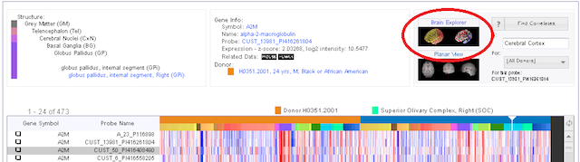
When the Brain Explorer 3-D Viewer opens, you will be taken to a screen that displays the Image Viewer, the Structure Ontology Viewer, and the Gene List.
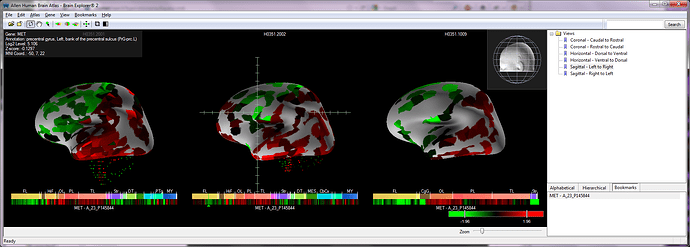
Image Viewer
The Image Viewer will automatically show the 3-D expression representations of your gene of interest on every sampled brain. Cortical gene expression is overlaid on an inflated white matter surface for each donor brain, with spots under the cortical surface representing gene expression in the subcortical regions of the brain. Under each representative brain is the heat map for the probe you selected. Clicking on that heat map will pinpoint the area in the brain from which the sample was taken.
The gene expression colors correspond to the settings in the Atlas with which you were viewing the original heat map. To change the gene expression representation, click on the “Gene” tab in the top left hand corner of your screen and choose either Z-score or raw colors.
A compass in the right hand corner of the image viewer depicted by a stylized head can be used to rotate the brains by clicking and dragging your cursor. You can look at a single brain by clicking on the magnifying glass above that brain. The magnifying glass will appear as you hover over the donor ID for each brain. You can also remove a brain by clicking on the “x” next to the magnifying glass.

To restore all views, choose Show All Views from the View menu. Choosing a data point, either by clicking on the heat map below the brain or on a brain region itself, will bring up the gene symbol, the location of the sample and the expression level and z-score in the top left hand corner of the Image Viewer.
You can zoom using either the wheel on your mouse or using the Zoom scroll bar in the lower right hand corner of the Image Viewer.
Structure Ontology Viewer
The Structure Ontology Viewer shows the entire collapsible ontology for the human brain including the color coding used by our expert annotation team to visualize structural boundaries. Two columns to the right of the ontology determine the type of data displayed in the Image Viewer. “A” represents annotation and when checked, will show a visual representation of that structure in the Image Viewer. “G” represents gene expression and when checked, will show gene expression in that structural domain.
The default organization for the Structure Ontology is the Hierarchical View, but if you are unfamiliar with the ontology, you can click on the Alphabetical View to see the structure list in alphabetical order.
The Bookmarks tab is a space where you can create and save favorite views of the brain. Several default views are already saved that will rotate the brain back into common viewing frames.
Gene List
This section displays the gene probes you have selected and downloaded in this session. When more than one gene probe has been downloaded, clicking on one probe will show its gene expression profile in the image viewer. Right clicking on the gene probe name will bring up a menu where you can view the gene detail page (Get Info), be taken to the Planar View of the probe (View Images) or copy the gene information for use in another application.
Using the Toolbar
| Button | Operation |
|---|---|
 | Selects cursor rotation tool mode |
 | Selects cursor pan tool mode |
| Selects cursor selection tool mode |
| Toggle Sagittal Atlas section viewing |
| Toggle Coronal Atlas section viewing |
| Toggle Horizontal Atlas section viewing |
| Centers the Viewer on the current pinpointed expression data point |
 | Turns on the clipping planes |
 | Toggles the Structure Ontology and Gene List View |
Advanced Features
Atlas Tab:
You can show opaque three dimensional structures of the brain by “showing” or “hiding” structures from this menu. The “Transparent” function allows you to see transparent views of the structures to view the anatomical relationships between them.
Selecting the sagittal, coronal or horizontal sections (or clicking on one of the section image buttons in the toolbar) will superimpose a single plane of the MRI images from each brain on your image space. These planes can be moved once the selection tool mode button in the toolbar is selected. Selecting “Show Annotation on Section” from this menu will color the MRI images according to the brain structure ontology.
Gene Tab:
When you have a gene selected, the Gene Tab menu allows to you to show all expression, hide all expression (for instance to then select a single structure) or toggle expression (for instance, unselect your region of interest then toggle to see expression in only that region).
You can also show or remove threshold controls and choose the visual representation of your data (raw data vs. z-score) from this menu.
To be taken to the gene detail page, select “Get Info”. To see the Planar View, choose “View Images”. These functions are also available by right-clicking on the gene name in the Gene List.
Clipping Planes:
When this function is selected, either by toggling the cutting tools button in the toolbar or selecting “Clipping Planes” from the View drop down menu, you can make coronal, sagittal or horizontal cuts in your view of the brain and related data. To cut in a particular plane, make sure the cursor is in selection tool mode, and then click and drag on the plane you are interested in clipping.
Troubleshooting
Windows
Graphics
If you are using a desktop computer, you should obtain drivers from the video card manufacturer. First, identify the video card. Go the Start menu and open the Control Panel. Open the Display control panel and go to the Settings tab. Click the Advanced button and go to the Adapter tab. Your video card vendor and model name will be displayed at the top of the window under Adapter Type. Please go to the manufacturer’s web site, locate the driver download, and follow the instructions on the website or included with the downloaded file.
If you are using a laptop computer, you will need to go to your laptop manufacturer’s web site to locate the latest video drivers.
You can also activate an alternate drawing mode in Brain Explorer. Go to the View menu and select Options. Check the Draw faster but at lower quality button and uncheck the Synchronize drawing with the monitor’s vertical refresh button. Set the Multisample setting to Off.
If you are using multiple video cards from different vendors, the 3D display may not work correctly on all attached monitors.
Uninstalling
Use the Add/Remove Programs control panel or the uninstall link in the Brain Explorer folder in the Start menu. Additional data that are not automatically uninstalled are located at the following locations:
Windows XP
Atlas data: C:\Documents and Settings\userid\Local Settings\Application Data\Allen Institute\Brain Explorer 2
User settings: C:\Documents and Settings\userid\Application Data\Allen Institute\Brain Explorer 2
Windows Vista and Windows 7
Atlas data: C:\Users\userid\AppData\Local\Allen Institute\Brain Explorer 2
User settings: C:\Users\userid\AppData\Roaming\Allen Institute\Brain Explorer 2
Proxy Settings
If you use a proxy server, Brain Explorer will use the proxy settings from the Internet Options control panel in the Windows Start menu. Please refer to the Windows documentation for help on proxy settings.
Mac
Uninstalling
Drag the Brain Explorer 2 icon to the trash. Brain Explorer generates the following files, which can also be dragged to the trash.
- ~/Library/Application Support/Brain Explorer 2
- ~/Library/Preferences/org.alleninstitute.BrainExplorer2.plist
Performance
If Brain Explorer is not running smoothly, first try to free up as much memory as possible by quitting all other open applications. You can also activate an alternate drawing mode. Go to the Brain Explorer 2 menu and select Preferences. Check the Draw faster but at lower quality button and uncheck the Synchronize drawing with the monitor’s vertical refresh button. Set Multisampling to Off.
Contact Us
If after reading this help file you still have questions or suggestions, please Contact Us.
Learn about Overview Of The Aging Dementia And TBI Project with comprehensive guides and examples from Allen Institute for Brain Science.
The Aging, Dementia & TBI study incorporates many disparate data modalities - histology, protein quantification, gene expression and clinical diagnoses - which makes visualizing relationships and correlations within the data challenging. To enable exploration of the data, we have created unique data snapshots with visualization that incorporates t-Distributed Stochastic Neighbor Embedding (t-SNE) Plots and Parallel Coordinate Plots. These snapshots are curated walk-throughs of the data as an entry for exploring the data.

Each image from this page links you to a subset of the data and describes, in story-form, possible interpretations of the data.
t-Distributed Stochastic Neighbor Embedding (t-SNE) Plots
This method of data visualization is a technique that reduces the complexity of multi-dimensional data to two dimensions. In each of the data snapshots, the data is embedded by a limited number of parameters and the data plot coupled to the parallel coordinate plot allows the color of the data points to be changed based on independent data parameters. In some of the examples, there is the option to alter the embedding of the data (by clicking on the check box above the radio button in the parallel coordinate plot. For more information on this data representation, please visit t-SNE – Laurens van der Maaten.
Clicking on one of the data points will lead to a specimen detail page where all data collected from this donor can be accessed.
Parallel Coordinate Plots

This data representation allows for n data modalities to be plotted against n distinct axes. For each of the snapshots, the data modality is listed above each axis with a radio button that enables coloring of the t-SNE and plots according to that parameter. Embedding of the data in the t-SNE plot can also be altered by clicking in the checkbox over an axis (when available). Each of the coordinate axes is equipped with a slider bar that enables a subset of that data to be highlighted. Hover over the axis to enable the slider function, then click and drag to limit the data represented. Excluded data points will be indicated by colorless circles.
Data Snapshots
Gender
This snapshot demonstrates the power of these visualizations using an obvious way to embed the data, genes specific to one sex or the other. In this example, the data were embedded by the top 10 genes enriched in expression in males and the top gene enriched in expression in females. This allows for an obvious separation of the dataset in the data space. With the data clustered by sex, querying other parameters, such as demographics, diagnoses and histopathology becomes a simple matter of coloring the dataset by that parameter (by clicking the radio button) and/or limiting samples using the slider bar for each axis.
Brain Regions
In this snapshot, the data were embedded by genes that are differentially expressed in each of the brain regions sampled. This lays out the differences between the cortex and hippocampus and highlights the expression similarities of the cortical regions. With this clustering, you can query region specific genes as well as other demographic, histopathological or diagnostic parameters.
White & Grey Matter
This snapshot embeds the data based on gene expression enhanced in the white matter over the grey matter and vice versa. Not surprisingly, distinguishing these tissues highlights markers for excitatory and inhibitory neurons in the cortex, and glial cells in the white matter. With this clustering, you can then query demographic, diagnostic and neuropathologic parameters.
Inflammation
The data in this snapshot were embedded by gene markers for inflammation and clustering in this manner allows for querying the data by protein concentration as well as other demographic, diagnostic or neuropathologic parameters.
Dementia
The data in this snapshot were embedded by the genes most differentially expressed in the hippocampus of donors given the diagnosis of dementia over those who had no such diagnosis. This data clustering allows you to explore relationships of some specific gene markers, as well as other diagnostic, demographic or neuropathologic parameters.
Traumatic Brain Injury
In this snapshot, the data were embedded by genes differentially expressed in the cortex of donors who self reported at least one traumatic brain injury (TBI) with a loss of consciousness vs controls. The data clustered in this manner can then be queried for other factors regarding TBI, as well as other neuropathologic, demographic or diagnostic criteria.
Neuropathology
In this snapshot, the data were embedded by the levels of two proteins known to be increased in the brains of patients inflicted with Alzheimer’s related dementia; phosphorylated tau, pTau, the form of tau present in neurofibrillary tangles, and the neurotoxic amyloid peptide αβ42, which is present in amyloid plaques. Clustering the dataset in this manner allows for querying the samples by other neuropathologic, demographic and diagnostic criteria.
Learn about Human Brain Atlas API with comprehensive guides and examples from Allen Institute for Brain Science.
The Allen Human Brain Atlas is a multimodal atlas of the human brain that integrates anatomic and microarray-based gene expression information. Microarray sampling sites (~400-1000 sites per brain) were identified by expert anatomists using cytoarchitectural information from multiple histological stains. Sampling site delineations in the high resolution histological images were subsequently mapped into each individual’s MR image space to provide 3-D anatomical context. All brains were also registered to MNI space to enable cross-individual comparisons.
From the API, you can:
Download expression values
Query the correlative and differential search services
Download MRI images
Experimental Overview and Metadata
RNA isolated from each sample area was hybridized to a custom Agilent 8x60k microarray chip to measure gene expression over the transcriptome. All least two different probes were available for 93% of genes. Probes were located on different exons as much as possible when multiple probes were available for a gene. For 60 genes, sets of tiling probes were designed.
Each sampling site was associated to a Structure by expert anatomists using cytoarchitectural information from multiple histological stains. Structures are organized hierarchically into a tree in which children structures are “parts of” their parent structure. Structures are assigned colors that visually emphasize the hierarchical relationships.
See the structure ontology page for more information.
Gene expression data for samples passing quality control are normalized to enable cross-comparison between batches of samples processed at different times or samples belonging to different donors. For more details on microarray data generation and processing see the Microarray whitepapers.
Normalized microarray expression values can be downloaded in several ways:
- From the web application Download page. Each zip file contains the normalized values for all probes and all samples for one donor )
- From the “Download this data” link below the heatmap in the web application.
- From the connected data service in the API
All experimental data from this study is associated with the “Human Brain Microarray” Product. All probe and sampling site information can be accessed through the API using RMA queries.
Example queries:
- All donors in the Product
- All sampling sites in the Product
- All microarray probes in the Product
- All microarray probes associated with gene prodynorhphin (PDYN)
- All samples associated with donor “H0351.2001” and the dentate gyrus
- Download an “raw” Aglient output file for one sample using the download-link (warning: large file)
Supplemental RNA-Sequencing Data
RNA-Sequencing (RNA-Seq) data were generated for a selected set of 240 samples (120 from each brain) representing matched cortical and sub-cortical regions across two brains (H0351.2001 and H0351.2002). The gene expression data (both raw and TPM counts) can be downloaded from the web application Download page.
Through a quantitative comparison of microarray and RNA-Seq data, a set of quality control metrics has been computed for each Agilent microarray probe which allows a user to filter out problematic probes or choose the most reliable probe for each gene. The probe metric table and metadata can be downloaded here.
Downloading Expression Values
Normalized expression values can be obtained by specifying:
- a list of probes
- a list of donors (optional), and
- a list of structures (optional)
See the connected service page for definitions of service::human_microarray_expression parameters.
Example:
Download expression values for donor “H0351.1015” in structure “locus ceruleus” for all probes associated with gene SLC6A.
- Find Donor ID for “H0351.1015” (id = 15496)
http://api.brain-map.org/api/v2/data/query.xml?criteria=model::Donor,
rma::criteria,[name$eq'H0351.1015'],
rma::options[only$eq'donors.id']
- Find Structure ID for “locus ceruleus” (id = 9148)
http://api.brain-map.org/api/v2/data/query.xml?criteria=model::Structure,
rma::criteria,[name$il'locus ceruleus'],ontology[name$eq'Human Brain Atlas'],
rma::options[only$eq'structures.id']
- Find Probes associated with gene SLC6A2 (id = 1023146,1023147 )
http://api.brain-map.org/api/v2/data/query.xml?criteria=model::Probe,
rma::criteria,[probe_type$eq'DNA'],products[abbreviation$eq'HumanMA'],gene[acronym$eq'SLC6A2'],
rma::options[only$eq'probes.id']
- Use Donor, Structure and Probe IDs as parameters to the connected service
http://api.brain-map.org/api/v2/data/query.json?criteria= service::human_microarray_expression[probes$eq1023146,1023147][donors$eq15496][structures$eq9148]
The output of the service is two top level ordered arrays “probes” and “samples”. For example:
"probes":[{
    "id":1023146,
    "name":"A_23_P358345",
    "gene-id":6494,
    "gene-symbol":"SLC6A2",
    "gene-name":"solute carrier family 6 (neurotransmitter transporter, noradrenalin), member 2",
    "entrez-id":6530,
    "chromosome":"16",
    "start-position":"n/a",
    "end-position":"n/a",
    "expression_level":["13.2802","13.9603","13.9650"],
    "z-score":["9.3381","9.8663","9.8700"]},
{
    "id":1023147,
    "name":"CUST_16472_PI416261804",
    "gene-id":6494,
    "gene-symbol":"SLC6A2",
    "gene-name":"solute carrier family 6 (neurotransmitter transporter, noradrenalin), member 2",
    "entrez-id":6530,
    "chromosome":"16",
    "start-position":"n/a",
    "end-position":"n/a",
    "expression_level":["8.1878","8.5644","8.2310"],
    "z-score":["9.3201","9.8326","9.3790"]}
],
"samples":[
    {"donor": {"id":15496,"name":"H0351.1015","age":"49 years","color":"C2C200"},
    "sample":
        {"well":148955246,"polygon":127107914,"mri":[95,121,126]},
        "structure":{"id":9149,"name":"locus ceruleus, Left","abbreviation":"LC","color":"00FFAA"},
        "top_level_structure":{"id":9135,"name":"Pontine Tegmentum","abbreviation":"PTg","color":"00FFAA"}},
    {"donor":{"id":15496,"name":"H0351.1015","age":"49 years","color":"C2C200"},
    "sample":
        {"well":148955204,"polygon":126786164,"mri":[97,151,131]},
        "structure":{"id":9149,"name":"locus ceruleus, Left","abbreviation":"LC","color":"00FFAA"},
        "top_level_structure":{"id":9135,"name":"Pontine Tegmentum","abbreviation":"PTg","color":"00FFAA"}},
    {"donor":{"id":15496,"name":"H0351.1015","age":"49 years","color":"C2C200"},
    "sample": {"well":156435966,"polygon":126789834,"mri":[96,159,134]},
        "structure":{"id":9149,"name":"locus ceruleus, Left","abbreviation":"LC","color":"00FFAA"},
        "top_level_structure":{"id":9135,"name":"Pontine Tegmentum","abbreviation":"PTg","color":"00FFAA"}} ]
Each probe contains information about:
- the Probe(id, name), and
- the Gene (id, acronym, name, entrez-id), along with
- a vector of normalized expression values in the same order as the “samples” array.
- a vector of z-score values in the same order as the “samples” array. Note: z-score is computed independently for each probe over all donors and samples.
Each sample contains information about:
- the Donor (id, name, age),
- the Sample (well id and (x,y,z) coordinate in the MR volume in millimeters),
- the associated Structure (id, name, acronym and color), and
- the associated top (coarse) level Structure (id, name, acronym and color).
Differential Search
The differential search function finds probes that show the greatest difference between two sets (target and contrast) of user-defined structures. For each probe, a 2-sample t-test is performed followed by Benjamini and Hochberg false discovery rate correction. The null hypothesis is that the average expression level of samples in the contrast set of structures is greater than or equal to the average expression level of samples in the target set of structures. A statistically significant result (p-value less than user-defined threshold) allows us to reject the null hypothesis and conclude that the average expression level of samples in the target set of structures is greater than the average expression level of samples in the contrast set of structures. Resulting p-values are sorted in ascending order. Search results can also be sorted by fold-change (log ratio of expression) in descending order.
The differential search function can be accessed through the Web application or using the API.
See the connected service page for definitions of service::human_microarray_differential parameters.
Example:
Differential search for genes with higher expression in thalamus than the cerebral cortex
- Find Structure ID for “thalamus” (id = 4392)
http://api.brain-map.org/api/v2/data/query.xml?criteria=model::Structure,
rma::criteria,[name$il'thalamus'],ontology[name$eq'Human Brain Atlas'],
rma::options[only$eq'structures.id']
- Find Structure ID for “cerebral cortex” (id = 4008)
http://api.brain-map.org/api/v2/data/query.xml?criteria=model::Structure,
rma::criteria,[name$il'cerebral cortex'],ontology[name$eq'Human Brain Atlas'],
rma::options[only$eq'structures.id']
- Use Structure IDs as parameters to the connected service
http://api.brain-map.org/api/v2/data/query.xml?criteria=service::human_microarray_differential
[structures1$eq4008][structures2$eq4392][sort_by$eq'fold-change']
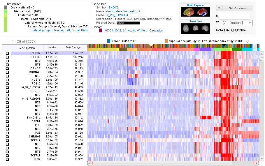
Usage of this service is demonstrated in the SPM example application.
Correlative Search
The correlative search function finds probes with expression profile similar to that of a selected seed probe over all samples within a user-specified structure. Pearson’s correlation coefficient is computed for all probes and the results ranked in descending order.
This correlative search function can be access through the Web application or using the API.
See the connected service page for definitions of service::human_microarray_correlation parameters.
Example:
Correlative search for probes with similar expression to PVALB probe CUST_11451_PI416261804 over the whole Brain
- Find Probe ID for probe “CUST_11451_PI416261804” (id = 1052410)
http://api.brain-map.org/api/v2/data/query.xml?criteria=model::Probe,
rma::criteria,[name$eq'CUST_11451_PI416261804'],
rma::options[only$eq'probes.id']
- Find Structure ID for “Brain” (id = 4005)
http://api.brain-map.org/api/v2/data/query.xml?criteria=model::Structure,
rma::criteria,[name$il'brain'],ontology[name$eq'Human Brain Atlas'],
rma::options[only$eq'structures.id']
- Use Probe and Structure IDs as parameters to the connected service
http://api.brain-map.org/api/v2/data/query.xml?criteria=service::human_microarray_correlation
[probes$eq1052410][structures$eq4005]
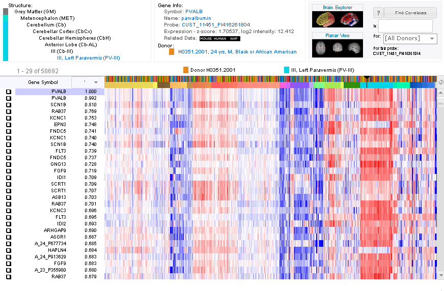
Magnetic Resonance Imaging
T1-weighted MPRAGE scans were acquired for the postmortem brains using 3T Siemens Trio MR scanners (TI=900ms, TR=1900ms, TE=3.03ms, 9 degree flip angle, 1mm isotropic voxels). Scans were performed in cranio for some brains and ex cranio for others. See the Microarray whitepapers for more specific scan sequence details for each brain.
The T1, T2 and DTI (if available) volumetric data can be downloaded from the Web application or via the API.
All T1 images were registered to MNI space. FreeSurfer’s affine registration was used for the in cranio scans. For ex cranio brains, the T1 was first rigidly aligned using FSL (Jenkinson, et. al, 2002) and then non-rigidly aligned using ANTS (Avants, et. al., 2011). The 3-D affine transform from a location in the MR volume to MNI space is encapsulated in the Alignment3d model.
Examples queries:
- Download links for all MR and DTI data available
http://api.brain-map.org/api/v2/data/query.xml?criteria=model::Donor,
rma::criteria,products[abbreviation$in'HumanMA','HumanSZ','HumanCtx','HumanSubCtx'],organism[name$il'Homo Sapiens'],
rma::include,specimens(well_known_files(well_known_file_type[name$in'T1-MRI','T2-MRI','DTI-MRI'])),
rma::options[only$eq'donors.name,products.name,well_known_files.download_link,specimens.id']
- Download TI MR scan for donor ‘H0351.2002’
http://human.brain-map.org/api/v2/well_known_file_download/157723301
- Download the MR to MNI transform parameters
http://api.brain-map.org/api/v2/data/query.xml?criteria=model::Donor,
rma::criteria,products[abbreviation$eq'HumanMA'],
rma::include,specimens[parent_id$eqnull](alignment3d),
rma::options[only$eq'donors.id,donors.name,specimens.id']
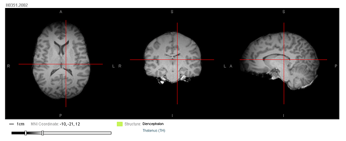
See example code on how to transform each microarray sample to MNI space.
Learn about Human Brain Atlas Microarray Data with comprehensive guides and examples from Allen Institute for Brain Science.
For those who are arriving at this database without prior knowledge of genetics or specific genes, a search by disease, pathway, cell type or function may be of most initial use. To do this, click on the relevant search term in the tag cloud.
The Allen Human Brain Atlas offers three types of searches to allow a user to: (1) obtain gene expression data for specific genes (or probes) of interest (Gene Search); (2) compare expression between different anatomic regions (Differential Search); and (3) use a ‘seed’ gene to find other genes with similar expression patterns (Find Correlates).
Gene Search
To search for probes associated with a specific gene or group of genes, select the Gene Search radio button and type the gene name, gene symbol, Entrez Gene ID or probe ID in the search box (multiple genes searches require an OR between gene names) before clicking the “Search” button. To show exact matches to your search query click the “Show exact matches only” box.
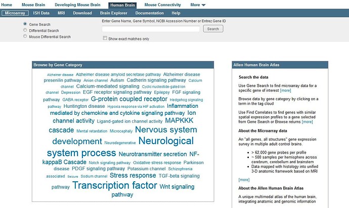
Boolean Syntax
The following special operators can be used to build queries:
OperatorExample Search TypeExample QueryAND operator: &Genedopamine & receptorOR operator: lGeneABATNOT operator: !Gene“dopamine receptor” !DRD3
- AND, OR and NOT may be used in place of their corresponding operators. They must be upper case.
- The AND operator (&) is implicit, so spaces between words that are not separated by an operator will be treated like an &.
- OR (|) has higher operator precedence than AND (&).
- Parentheses can be used to group criteria, but nested parentheses are not supported at this time.
- The NOT operator (!) is not supported within parentheses.
To download your search results, click the “Download this data” link at the bottom left of the heatmap.
Differential Search
To find genes that show enrichment of expression in one region compared to another region, use the Differential Search mode. Select the “Differential Search” radio button. To find genes or probes with an enhanced gene expression profile in one or more brain regions when compared to one or more other brain regions by entering the target structure(s) in the top search box (separate structures with a semicolon) and your contrast structure(s) in the bottom search box and click the Search button.

The search returns will show genes exhibiting higher expression in the target region(s) compared to the contrast region(s).Search results are sorted either by p-value or fold change, indicated by the arrow on the buttons over the column of genes. To alter the sort parameter, click on either the “p-value” or the “fold change” button.
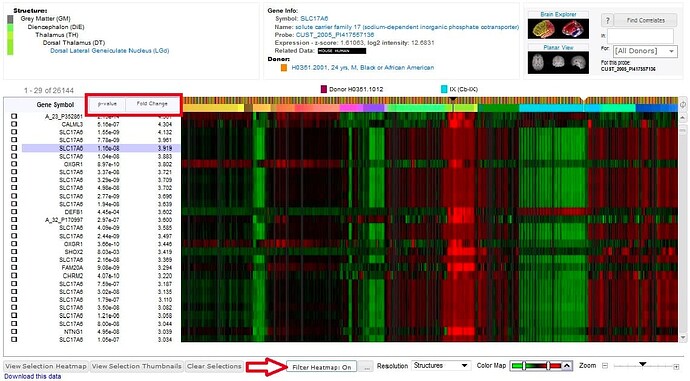
To filter your results by structure or by donor, click on the “Filter Heatmap” button below the heatmap.
To perform the previous search in reverse, click the toggle button to the left of the Search button. To download your search results, click the “Download this data” link at the bottom left of the heatmap.
Mouse Differential Search
The “Mouse Differential Search” function enables side by side viewing and comparison of differential search across the human microarray and the mouse ISH datasets. Select the “Mouse Differential Search” radio button. To find genes with higher expression in one structure compared to another structure, select a target brain structure in the top drop-down box and a contrast region in the bottom drop-down box and click on the Search button.
Search Results
The return list is generated by first executing a differential search query in the human microarray dataset. Experiments for each gene are grouped together and ordered by maximum fold-change. For each gene in the human microarray return list, associated experiments in the mouse ISH dataset are identified; fold-change values are computed and displayed. Note that NCBI HomoloGene data is used to link genes across organisms. Click on the dataset column heading to toggle the primary dataset selection.
For each experiment, a gestalt visualization of the brain wide expression pattern is also provided. The type of visualization depends on the dataset:
For mouse brain data, expression is visualized as rotating 3D thumbnails. Each view is generated by maximum density projection where denser expression area appears more solid and obscures areas of lower density. Each cube is color-coded by average expression intensity ranging from blue (low intensity) through green to red (high intensity). Move slider bar in the header to rotate thumbnail.
For human brain data, microarray data is visualized as a heatmap where each column represents a tissue sample in ontological order. Heatmap color represents the z-score over a probe ranging from green (z-score of -3 and below) through black to red (z-score of +3 and above). Hover over any position in the heatmap to obtain the associated tissue sample structural annotation.
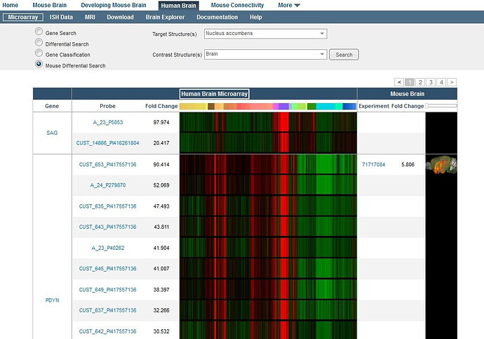
Gene Classification
When you are viewing heatmap data, there will be a “Gene Classification” radio button available. When the gene classification radio button is selected, you can search for enhanced gene expression from one of the categories in the drop down menu.
To download your search results, click the “Download this data” link at the bottom left of the heatmap.
Correlative Search
In using gene expression databases, a “search by example” feature is also highly desirable as genes with similar expression patterns may be related in function. The Find Correlates search utility will accomplish this function. This search by example facility is also available in the Allen Mouse Brain Atlas, Allen Developing Mouse Brain Atlas and the BrainSpan atlas of the developing human brain.
Once you have identified a gene of interest, to find other genes with spatial expression profiles similar to your gene of interest, first select your probe by clicking on any cell in the heat map related to that probe. You will see that probe listed in the box above the right hand side of the heat map. Then select the brain structure(s) in which you would like to see a similar expression pattern, and click “Find Correlates”. This action will return probes with a similar expression profile to brain region(s) in which you are interested.
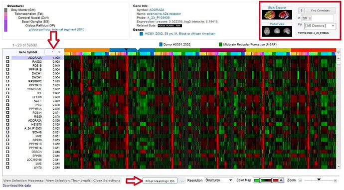
You can see “anti-correlated” returns by toggling the sort order on column “r” or scrolling to the bottom of the heatmap.
You can show less data by turning on the “Filter Heatmap” which will bring up a menu that will allow you to select the donors and structures you’d like to see represented in the heatmap.

You can see “anti-correlated” returns by toggling the sort order on column “r” or scrolling to the bottom of the heatmap.
To download your search results, click the “Download this data” link at the bottom left of the heatmap.
Download Search Results
To download your search results, click the “Download this data” link at the bottom left of the heatmap. You will have the option of downloading up to 2000 genes at a time starting from any position in the heatmap. Your start position can be determined from the counter in the top left corner of the heatmap (see screenshot).

Your data will be downloaded as three separate files: 1) a Columns.csv file that lists the column headers with associated metadata for each sample, 2) a Probes.csv file that lists the row headers with associated metadata for each probe, and 3) an Expression.csv file that provides a matrix of the expression values for each data point.
The column headers, probe headers and expression data will be consistent with the settings from which you downloaded the heatmap (i.e. heatmaps illustrating z-score will result in an Expression.csv file with normalized z-score values).
Data Visualization
Based on your search, the resulting microarray datasets are presented as a matrix with brain structure (by individual donor) on the horizontal x-axis and gene probes on the vertical y-axis. Because multiple probes were used to measure gene expression for a gene, search returns are reported by probe rather than by gene. The microarray data is presented in a heatmap format where the colors of the heat map correspond either to raw data or to a normalized (z-score) expression level of a probe. Brain structures are organized such that moving left to right on the x-axis is analogous to moving from anterior to posterior first in the cortical areas, followed by subcortical areas, cerebellum and brainstem.
In the top right hand corner of the heat map is a toggle button (see below), which when clicked will sort the heat map data either by donor or by structure.

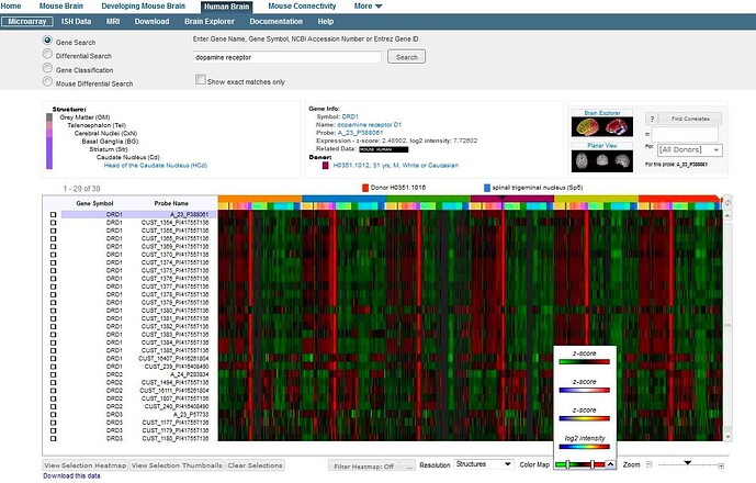
Data Aggregation and Normalization
Unless viewing data on the lowest possible resolution, the heat maps presented on this site are based on data aggregated within brain structures. That is, when there are multiple samples for a given structure, the value represented in the heat map will be the average of those sample values.
We further aggregate the expression values up the ontology tree, eg. Frontal Lobe will have a single averaged expression value, which is the average value for all samples belonging to the frontal lobe.
Data represented in the heatmap have been normalized across the entire dataset before they are aggregated, and are normalized again for each probe when the heatmap is constructed.
Heat Maps
The heatmap is a visualization of the microarray values for the returned probes of interest. Each row of the heat map represents a probe. Each column of the heat map either represents a tissue sample or anatomical brain structure depending on the selected resolution (see below). The colors of the heat map are normalized expression values. Default heat map colors are in the green-red scale where the color green should be interpreted as relatively low expression and red as relatively high expression within the scope of each probe.
The color scheme used for the heat map display can be changed to suit the user. You can use the color map bar at the bottom of the heat map to display different normalized (z-score) color representations of the heat map data (i.e. blue-red vs. green-red) or you can visualize log2 normalized expression map where the color scale ranges from dark blue, representing low expression, and passes through cyan, yellow, orange and finally to dark red, representing high expression.
The columns of the heat map have different meanings depending on the selected resolution. There are three resolution options available from the drop-down menu under the heat map: Coarse, Structures and Samples. If “Samples” is selected there is a one-to-one correspondence between a column and a physical tissue sample. In the Atlas, there are typically multiple samples for each structure of interest. This oversampling may provide information on variability and spatial gradients. In “Structures” mode, all samples belonging to the same designated structure are combined and averaged together. In “Coarse” mode, the brain is divided into approximately 20 large neuroanatomic divisions or regions (e.g. frontal lobe, occipital lobe, striatum, dorsal thalamus, ventral thalamus). Samples within each partition are averaged together to provide a summary value for the partition.
Clicking on a cell of the heat map will bring up detailed information in the area above the heat map. The selected location will be indicated by a black arrow above the heat map. The current location of the cursor will be indicated by the white arrow.
In the panel above the heatmap (see image below), information about the sampled anatomical structure is displayed on the left. The stack of structures represents the hierarchy from the structure ontology. Clicking on the link at the bottom of the structure ontology will open up the Interactive Atlas Viewer. For more details on the ontology see the Ontology and Nomenclature whitepaper in the Documentation tab.
Additional information is shown in the middle panel, and includes gene symbol, gene name, probe name, the log2 expression value and z-score and links to related data in other Allen Brain Atlas resources. Links to donor meta-data are also included in this panel. Blue text indicates a hyperlink, where there is more information available by clicking on the text.
The “Brain Explorer” link, when selected for the first time, will take you to a page where you can download the Brain Explorer® 2 3-D viewer software. Once the Brain Explorer program is loaded, clicking on the “Brain Explorer” icon will launch a desktop software application for viewing the Atlas gene expression data in three dimensions.

The “Planar View” icon launches the multiplanar viewer that shows the expression profile for the selected probe in the context of the donor brain.
Data from multiple brains may be viewed in two ways. By default, columns are grouped first by donors then by structures, allowing a user to compare the full expression profiles of the individual brains side-by-side. Grouping the columns initially by structures then by donors allows a user to view the data for each brain structure with data form all donors grouped side-by-side under that structure. You can toggle between the two groupings by clicking the toggle button over the scroll bar.
Comparing Genes of Interest
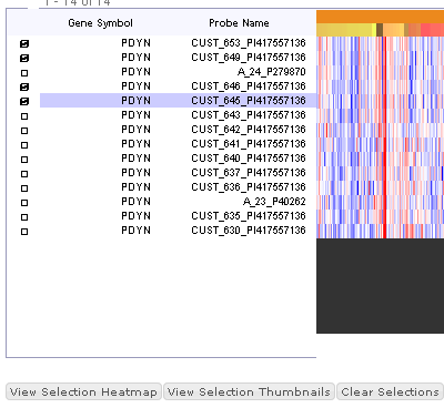
You can add probes of interest to a collection for later viewing. Check the checkbox at the left end of a search result row to add it to your collection. Your choices are stored in a browser ‘cookie’ on your computer and will remain in effect until you click the “Clear Selections” button, or clear your Web browser’s cookie cache.
Click the “View Selection Heatmap” button to see all of your selections as a heat map. Alternatively choose “View Selection Thumbnails” to view your selection as 3-D rotating thumbnails.

In “Thumbnails” mode each row represents a probe with data from each donor arranged from left to right. The color patches in the thumbnail represents a physical tissue sample using the same user-specified color scheme as for heatmap viewing. Clicking on a patch will turn it bright blue and bring up detailed information in the area above the thumbnails. To rotate the thumbnail, drag the black downward triangle on the slider labeled “Rotate”. You can switch between viewing left cortical, right cortical and sub cortical samples using the “Left Cortex”, “Right Cortex” and “Subcortex” buttons located above the thumbnails. Cortical samples projected on a standard inflated white matter surface while sub-cortical samples are displayed as spheres in their 3D sampling locations.
Please note that this feature requires that you have cookies enabled in your browser, which is already the case for the great majority of users.
Gene/Probe Detail
Under Gene Info, clicking on the Gene Symbol, Gene Name or Probe of your search results will take you to a gene detail page.
The microarray gene detail page displays information about the gene (1) including the gene name, aliases, Organism, related data from other Allen Brain Atlas resources, Entrez Gene ID and Chromosome. It also includes Probe metadata (2) including the Probe name, NCBI accession number, sequence length, probe sequence, probe type, transcript GI and GC percentage is also included.
Given the discrete nature of the sample collection in these brains, we have visually represented gene expression by structure for each donor and for each probe. You can select probes either by choosing a probe from the drop-down menu or you can click through the pages, each of which outlines a single probe.
For each probe, we have provided an anatomical abstract view of the gene expression pattern of each donor. Regions of the brain are listed in each of the views, and the text can be removed by clicking on the ‘Labels’ button. The cortical gene expression patterns (3) are displayed on an inflated cortical surface (outer and inner surfaces of the left hemisphere). Subcortical structures of the brain are represented from a frontal view (4), and subcortical as well as brainstem structures are shown in a side view (5). Hovering your mouse over an annotated structure will bring up the structure name as well as the normalized and raw expression level values. Clicking on a structure will bring up links to the Multiplanar Viewer and the Brain Explorer.
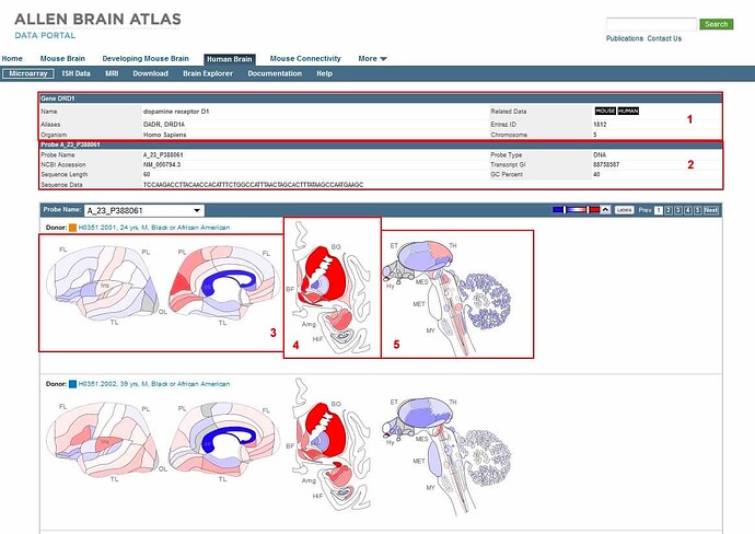
Multiplanar Viewer
The Planar View link opens a multiplanar viewer that shows sampling sites for microarray data and indicates gene expression levels for a single probe in coronal, sagittal and horizontal sections of MRI space for a given specimen. Additional viewing frames show spatially-corresponding histological data at the slab and block levels with anatomic annotations and specific delineations of sampling sites for microarray data generation.
Multiplanar Navigation
This screenshot shows the multiplanar navigation controls. Samples from which microarray tissues were assayed are represented as colored boxes on the MR images and show expression level, according to the active color map. Instead of the MR image, you can select a 3-D thumbnail showing the cortical gene expression.
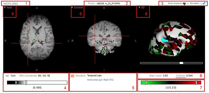
Click or click-and-drag to move the crosshairs on any of the three MRI views ports.
The various control and feedback components are labeled here 1 - 8:
- Donor: Identification number of the donor currently displayed in the viewer.
- Probe Name: The label for the probe currently displayed in the viewer.
- Brain Explorer software Link & Permalink: Click the “Brain Explorer” link to view this gene in the Brain Explorer 3-D viewer. Click the permalink component to generate a URL that will bring you back to this page with the current location settings.
- Scale, MNI Coordinates & Contrast: Scale bar, MNI coordinates at the crosshairs. Click and drag to move the contrast control.
- Brain Structure: This field is updated to indicate the structure under the crosshairs. Click on the structure label to launch the ontology browser in a new window.
- Expression Level: This component reports both the raw expression value and its z-score normalized value.
- Color Map Window & Level: adjust the upper & lower bounds, or slide the entire control to modify the range of colors used to map expression levels.
- MRI or Gene Expression Thumbnail View: choose the corresponding MR image or gene expression view from the drop-down menu.
Image and Probe Navigation
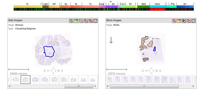
In this screenshot you see the heat map associated with a single, user-defined probe of interest as well as two image viewers illustrating the 2-D histology associated with the point selected by the MRI cross-hairs. The viewer on the left-hand side shows a larger view of the relevant brain slab, with a blue highlight around the block of that slab from which the selected sample was taken. The viewer on the right-hand side shows a detailed view of that block, with structure annotations visible. An arrow on the left hand side of the viewer indicates which direction is dorsal (top of the head).
The strip of thumbnail images at the bottom of each viewer shows all of the images from its parent specimen, in sectioning order. Clicking on a thumbnail image in the left-hand viewer will navigate the heatmap and the MRI crosshairs to the current location as well as opening a new set of images in the right-hand viewer. Click on one of the structures to move the MRI crosshairs to the location where that structure was sampled. As you move your mouse over the structures in the right-hand viewer its name will appear in the upper-left corner of the viewer.
Navigation tools on each viewer allow you to zoom and pan the individual images using your mouse.
The toolbar icons provide more detailed views of the tissue sections:
| Icon | Function |
|---|---|
 | Add or remove annotated structure outline |
 | Add or remove annotated structure colors |
 | Show all sections from this specimen |
 | Show block-face images |
 | Launch Single Image Viewer in another window |
Learn about Human Brain Atlas Magnetic Resonance Images MRI with comprehensive guides and examples from Allen Institute for Brain Science.
MRI Viewer
Select the MRI tab to view the Microarray Specimen MRI page, or click on a Donor link over the microarray heatmap or in the Gene Detail or Probe Detail pages.
The Microarray Specimen MRI page displays axial, coronal and sagittal planar MR images of the selected donor brain. Drag the red axes in order to change the view coordinates. Donor information includes Age, Sex, Ethnicity and Postmortem Interval (PMI).
The MRI data files are available for download in NIFTI format by clicking on the T1, T2 and DTI links.
Learn about Cell Types Database API with comprehensive guides and examples from Allen Institute for Brain Science.

The Allen Cell Types Database provides multimodal single cell characterization data to enable data-driven approaches to cell type classification.
From the API, you can:
Download electrophysiology data in Neurodata Without Borders (NWB) format
Download computed electrophysiology features
Download cell morphology images
Download morphological reconstructions in SWC format
Download computed morphology features
Download neuronal models trained on this data set
This document provides a brief overview of the data, database organization and example queries. API database object names are in camel case. See the main API Documentation for more information on data models and query syntax.
The accompanying Allen Software Development Kit (SDK) provides python code for accessing electrophysiology data (NWB files) for all cells and morphological reconstructions (SWC files) for a subset of cells. The Allen SDK also provides sample code demonstrating how to download neuronal model parameters and run your own simulations using stimuli for the experiments or custom current injections.
Experimental Overview And Metadata
All data used in the web application is available in the ApiCellTypesSpecimenDetail table. Data includes structure, cortical layer, dendrite type (spiny, aspiny, sparsely spiny, n/a), apical dendrite status (intact, truncated, n/a), and others. Mouse-specific records include the transgenic line name and reporter status. Mouse-specific records include disease condition (epilepsy, tumor, none) and years of seizure history.
See whitepapers for detailed experimental and annotation information.
From the API, detailed information about cells can be obtained using RMA queries.
Examples:
- All cells in the database
http://api.brain-map.org/api/v2/data/query.xml?criteria=
model::ApiCellTypesSpecimenDetail
,rma::options[num_rows$eqall]
- All cells tagged with ‘dendrite type - spiny’
http://api.brain-map.org/api/v2/data/query.xml?criteria=
model::ApiCellTypesSpecimenDetail
,rma::criteria,[tag__dendrite_type$eq'spiny']
,rma::options[num_rows$eqall]
- All cells annotated to be in layer 4
http://api.brain-map.org/api/v2/data/query.xml?criteria=
model::ApiCellTypesSpecimenDetail
,rma::criteria,[structure__layer$eq'4']
,rma::options[num_rows$eqall]
- All human cells
http://api.brain-map.org/api/v2/data/query.xml?criteria=
model::ApiCellTypesSpecimenDetail
,rma::criteria,[donor__species$il'homo sapiens']
,rma::options[num_rows$eqall]
- All human cells with disease condition ‘epilepsy’
http://api.brain-map.org/api/v2/data/query.xml?criteria=
model::ApiCellTypesSpecimenDetail
,rma::criteria,[donor__disease_state$il'epilepsy']
,rma::options[num_rows$eqall]
Electrophysiology
All cells in the Allen Cell Types Database have electrophysiological recordings of responses to stimuli from a common set of current injection protocols. See the electrophysiology overview whitepaperfor details on specimen selection, tissue processing, recording, and quality control.
The Cell Types Database categorizes detailed stimulus protocols into set of high level descriptions:
Stimulus sweeps that pass quality control standards are available for download as Neurodata Without Borders (NWB) files. To find the NWB download link for Rorb cell specimen 320654829, use this query:
http://api.brain-map.org/api/v2/data/query.xml?criteria=
model::Specimen
,rma::criteria,[id$eq320654829]
,rma::include,ephys_result(well_known_files(well_known_file_type[name$eqNWBDownload]))
The Allen SDK provides a simple Python module to support downloading metadata and NWB files for cells in the Cell Types Database. Please see the Data API Client documentation page to see an example.

A standard set of electrophysiological features are automatically computed from the recorded responses of each cell. A subset of those features are displayed at the top of the electrophysiology page for a cell:
See the electrophysiology overview whitepaper for a complete list of computed features and their interpretations.
Use this query to download the features computed for Scnn1a cell specimen 467703703:
Morphology
The Allen Cell Types Database contains morphological reconstructions generated from bright-field images of biocytin-stained cells. Reconstructions are generated by manually curating the results of an automated segmentation algorithm. See the morphology technical whitepaper for more details.
A standard set of morphological features were computed for all reconstructed cells. A subset of those features are displayed at the top of the cell-specific morphology page:
See the morphology technical morphology technical whitepaper for a complete list of computed morphological features.
The API provides programmatic access to the microscopy images used for reconstruction, axis-oriented projections of those images, and morphological reconstructions. A cell can have up to four axis-oriented projections of the images used for reconstruction:
- XY minimum intensity projection
- YZ minimum intensity projection
- XY maximum intensity projection
- YZ maximum intensity projection
The reconstruction images display a dark, biocytin-filled cell on a light background. The maximum intensity projections are constructed from inverted and contrast-enhanced versions of the morphology images, resulting in a light cell on a dark background.
Examples:
- Find projection image IDs for layer 4 spiny cell (Specimen 313862022):
http://api.brain-map.org/api/v2/data/query.xml?criteria=
model::ProjectionImage
,rma::criteria,[specimen_id$eq313862022]
- Download a projection image from its ID
http://api.brain-map.org/api/v2/section_image_download/323637357
- Find all images used for reconstruction for a layer 4 spiny cell (Specimen 313862022)
http://api.brain-map.org/api/v2/data/query.xml?criteria=
model::SubImage
,rma::criteria,data_set[specimen_id$eq313862022]
- Download an image from the image stack
http://api.brain-map.org/api/v2/section_image_download/321549675
- Find all cells with morphological reconstructions
http://api.brain-map.org/api/v2/data/query.xml?criteria=
model::ApiCellTypesSpecimenDetail
,rma::criteria,[nr__reconstruction_type$nenull]
- Find the reconstruction file for one of those cells
http://api.brain-map.org/api/v2/data/query.xml?criteria=
model::NeuronReconstruction
,rma::criteria,[specimen_id$eq313862306],rma::include,well_known_files
- Download the reconstruction file
http://api.brain-map.org/api/v2/well_known_file_download/491119517
- Download all of the morphology features for Scnn1a cell 313862022
http://api.brain-map.org/api/v2/data/query.xml?criteria=
model::NeuronReconstruction
,rma::criteria,[specimen_id$eq313862022]
Single Cell Neuronal Models
The Allen Cell Types Database contains two types of neuronal models: perisomatic biophysical models and generalized leaky integrate-and-fire (GLIF) models. These models attempt to mathematically reproduce a cell’s recorded response to a current injection. The perisomatic biophysical models take into account dendritic morphological structure, whereas GLIF models are simple point neuron models which represent the neuron as a single compartment.
There are five levels of GLIF models with increasing levels of complexity. The most basic model is a simple leaky integrate-and-fire equation. More advanced GLIFs attempt to model variable spike threshold, afterspike currents, and threshold adaptation.
See the perisomatic biophysical and GLIF technical whitepapers for more details on how these models were created.
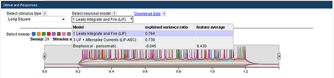
A cell’s electrophysiology page displays all available models. Choose a model to see its simulated response to all stimuli presented to the cell. If the required sweeps are available, two model evaluation metrics are computed per model:
After selecting a model for display, the models ID number and a link for downloading necessary to run the model are available. For example, the link to download model 566296565 (a LIF model for Scnn1a cell 467703703) looks like this:
http://api.brain-map.org/neuronal_model/download/566296565
All models in the Allen Cell Types Database are available for download and local execution via the Allen Software Development Kit (SDK). The biophysical models require NEURON to be run, which the SDK helps to configure. The GLIF simulation module comes as part of the Allen SDK. Please visit the Allen SDK page for more details.
Examples:
- Find all cells with perisomatic biophysical models
http://api.brain-map.org/api/v2/data/query.xml?criteria=
model::ApiCellTypesSpecimenDetail
,rma::criteria,[m__biophys_perisomatic$gt0]
- Find all cells with GLIF models
http://api.brain-map.org/api/v2/data/query.xml?criteria=
model::ApiCellTypesSpecimenDetail
,rma::criteria,[m__glif$gt0]
- Download all GLIF models for Scnn1a-Tg3 cell 469803127
http://api.brain-map.org/api/v2/data/query.xml?criteria=
model::NeuronalModel
,rma::critera,[specimen_id$eq469803127],neuronal_model_template[name$il'*LIF*']
- Download the files necessary to run simple LIF model 566302806
http://api.brain-map.org/neuronal_model/download/566302806
- Allen SDK documentation for how to run simple LIF model 566302806
http://alleninstitute.github.io/AllenSDK/glif_models.html#downloading-glif-models
- Link to the electrophysiology page for Scnn1a-Tg3 cell 469803127
http://celltypes.brain-map.org/mouse/experiment/electrophysiology/469803127Learn about Documentation Aging Dementia And TBI Project with comprehensive guides and examples from Allen Institute for Brain Science.
Available Files
Learn about Human Brain Atlas Microarray Data Download with comprehensive guides and examples from Allen Institute for Brain Science.
Download Page
The available options for downloading the microarray data include downloading the entire normalized data set for each brain by clicking on the text links in the box (as seen in the image below), or using the XML or CSV link to download the individual raw microarray data files.
Download of RNASeq data for 240 samples is also available.
You can also download the archived normalized microarray expression values that utilized an earlier normalization method from prior to the March 2013 data release.
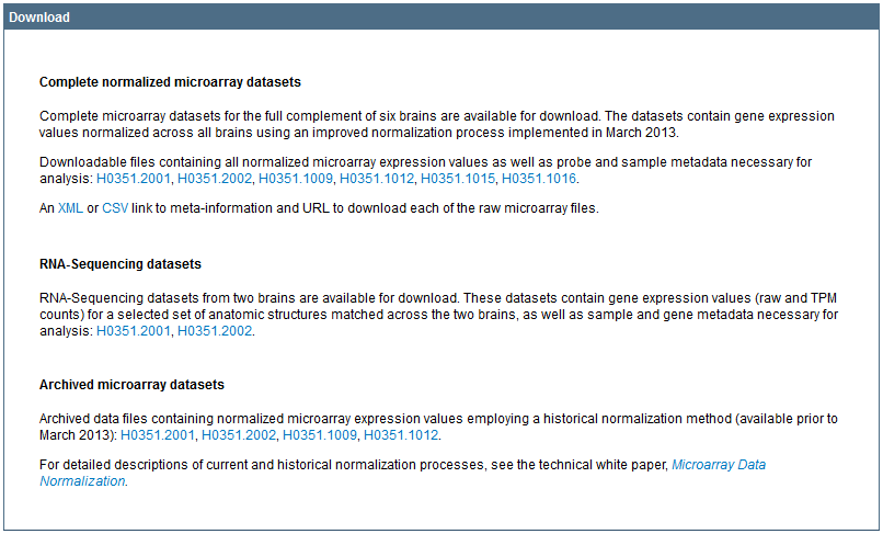
Learn about Allen Developing Mouse Brain Atlas Brain Explorer R 3D Viewer with comprehensive guides and examples from Allen Institute for Brain Science.
Brain Explorer® 3-D Viewer is an application for viewing brain anatomy and gene expression data in three dimensions in the framework of the Allen Developing Mouse Brain Reference Atlas.
Using Brain Explorer, you can:
- View fully interactive versions of the Allen Developing Mouse Reference Atlases in 3-D.
- View gene expression data in 3-D at 200 µm 3 resolution.
- View expression data from multiple genes superimposed on each other in 3-D.
- Navigate the high-resolution 2-D ISH images using the 3-D model.
- Link to associated gene metadata on the Allen Developing Mouse Brain Atlas web application.
Installation
Windows
Systems requirement: minimum configuration
- Operating System: Microsoft Windows 7
- CPU: Intel Core Duo or AMD 1.8GHz
- System Memory: 1GB
- Graphics Card: Hardware 3D OpenGL accelerated AGP or PCI Express with 64MB RAM
- Screen: 1024x768, 32-bit true color
- Hard Disk: 200MB free space
Note: Brain Explorer is known to work with the following video chipsets: nVidia GeForce 9400/9600, nVidia Quadro FX 1800/3800/5600, AMD Radeon 9600, AMD Radeon HD 3200/4550, Intel Q35/Q45 Express.
For the best performance, please check with your video card vendor for the latest available drivers before using Brain Explorer. The Windows version of the Brain Explorer viewer is available here. Double-click the downloaded BrainExplorer2.msi file and follow the prompts.
Mac
Systems requirement: minimum configuration
- Operating System: OS X 10.6.8
- CPU: Intel 1.8GHz
- System Memory: 1GB
- Graphics Card: 3D-capable with 64MB RAM
- Screen: 1024x768, 32-bit millions of colors
- Hard Disk: 200MB free space
Note: Please install the latest system updates from Apple to ensure you have the latest video card drivers.
The Mac version of the Brain Explorer viewer is available here. Double-click the downloaded zip file to unpack Brain Explorer.
Installing Atlases
A one-time download containing anatomy files is needed following installation of the Brain Explorer application. The first time you open the Brain Explorer software, you will be asked to choose to download files for the Allen Mouse and Allen Human Brain atlases. Click on the atlases you would like to use and then click the Install button.
To download missing atlases on the PC, go to the Help menu and select Download Atlases. On the Mac, the command is in the Brain Explorer 2 menu.
Getting Updates
The Brain Explorer application will inform you when updates to the Brain Explorer application itself or its atlases are available. New data may not be available for viewing until you install the required updates.
Viewing Gene Expression
To load gene expression data into the Brain Explorer viewer: go to the Allen Developing Mouse Brain Atlas and perform a search. Your search brings back a list of genes that fit your search criteria. Click on a gene name to select a gene of interest. 3-D thumbnails at all developmental stages of the gene expression pattern from that gene will load to the right. Click on the blue “View in 3D” link to launch the Brain Explorer application and load each experiment.
When the Brain Explorer 3-D Viewer opens, you will be taken to a screen that displays the Image Viewer, the Structure Ontology Viewer, and the Gene List.
Image Viewer
The Image Viewer will display the gene expression representations in 3-D for your gene of interest across all stages. Each stage will default to separate color schemes for each developing stage. For each developing stage, a sphere represents expression re-sampled to a grid resolution that is dependent on the stage in question (see the Informatics Data Processing whitepaper available in the Documentation. Larger spheres correspond to a greater density of expression in that voxel.
You can filter the developmental stages by hovering your mouse over the age to bring up an “X” or a magnifying glass. Clicking on the “X” will close that experiment, clicking on the magnifying glass will remove all the other stages from the viewer.
You can select a sphere by clicking on it. Spheres can be deselected by clicking on blank space. The original ISH image of the selected sphere will be displayed blended with the expression heat mask in the lower left-hand portion of the screen. The blending can be adjusted by selecting Image Controls from the View menu and moving the Image Blending slider. Clicking on the arrow in the top right-hand corner of the zoomed ISH image will open the corresponding ISH image in a high resolution image viewer.
The information at the upper-left corner of the main Brain Explorer window summarizes the expression detected in the selected grid location. These numbers include the average expression density and intensity (over pixels). The Informatics Data Processing White Paper describes how the measurements were obtained.
To change the gene expression representation, click on the “Data” menu and select an option under “Raw” colors.
A compass in the right-hand corner of the Image Viewer can be used to rotate the brain(s) by clicking and dragging your cursor. You can zoom using either the wheel on your mouse or using the Zoom scrollbar in the lower right-hand corner of the Image Viewer.
Expression Thresholds
A way to control expression visibility is by setting thresholds on expression values. This method can restrict visible spheres to different combinations such as low intensity and low density or high intensity and low density.
The graph in the lower right-hand corner shows a dot for each data point (sphere) in a gene expression file, and the color of the dot corresponds to the anatomic annotation in the same way the atlas colors display mode works. Each data point is plotted according to its density on the x-axis and its intensity on the y-axis.
The color scale on the left-hand side of the graph corresponds to the expression level heat map used to color the spheres, color coded to the reference atlas structures. The numbers along each axis show the values at the yellow triangles.
The thresholds can be changed by resizing the white box. Any edge or corner of the box can be clicked and dragged to re-size it. You can also click and drag in the center of the box to move the box.
Structure Ontology Viewer
The Structure Ontology Viewer shows the entire collapsible ontology for the developing mouse brain as defined by the Allen Developing Mouse Reference Atlas. The first column represents the color of the reference atlas for that structure. The two columns to the right determine the type of data displayed in the Image Viewer. “A” represents atlas structure and when checked, will show a visual representation of that structure in the Image Viewer. “D” represents gene expression and when checked, will show gene expression in that structural domain.
The default organization for the Structure Ontology is the Hierarchical View, but if you are unfamiliar with the ontology, you can click on the Alphabetical View to see the structure list in alphabetical order.
The Bookmarks tab is a space where you can create and save favorite views of the brain. Several default views are already saved that will rotate the brain back into common viewing frames.
Gene List
This section displays the experiments you have selected and downloaded in this session. Right clicking on the gene name will bring up a menu where you can, 1) view the gene detail page (Get Info), 2) be taken to a zoomed in image from this experiment (View Images), 3) copy meta information to the clipboard, such as symbol, name, Entrez ID, image-series ID (Copy Info), 4) activate a Correlation search by finding experiments with similar expression profiles (Find Similar) or 5) close the experiment and remove it from the list and the 3-D view (Close).
Gene Search
To search for genes within the Brain Explorer application, go to the Search box located above the ontology panel and type in the gene symbol or part of a gene name.
The list of results shows gene name, gene symbol along with a 3-D summary thumbnail of the expression for each experiment matching the search. The expression thumbnail represents a maximum expression projection rendering: the denser the expression in a region the more “solid” the appearance. Reference atlas colors are additionally layered on top.
To load an experiment for viewing, click on the “Download” button under the gene name.
Toolbar
| Button | Operation |
|---|---|
| Selects cursor rotation tool mode |
| Selects cursor pan tool mode |
| Selects cursor selection tool mode |
| Toggle Sagittal Atlas section viewing |
| Toggle Coronal Atlas section viewing |
| Toggle Horizontal Atlas section viewing |
| Centers the Viewer on the current pinpointed expression data point |
| Turns on the cutting planes |
| Toggles the Structure Ontology and Gene List View |
Advanced Features
Atlas Menu:
You can show opaque three dimensional structures of the brain by “showing” or “hiding” structures from this menu. The “Transparent” function allows you to see transparent views of the structures to view the anatomical relationships between them.
Selecting the sagittal, coronal or horizontal sections (or clicking on one of the section image buttons in the toolbar) will superimpose a single plane of the reference images (Nissl or Feulgen-HP) from each brain on your image space. These planes can be moved once the selection tool mode button in the toolbar is selected. Selecting “Show Annotation on Section” from this menu will color the reference images according to the brain structure ontology.
Data Menu:
When you have a gene selected, the Data menu allows you to show all expression, hide all expression (for instance to then select a single structure) or toggle expression (for instance, unselect your region of interest then toggle to see expression in only that region).
You can also show or remove threshold controls and choose the visual representation of your data from this menu. There are several options under “Raw” colors:
- User defined: Each experiment is rendered in user specified color. This mode is useful to distinguish between individual experiments when multiple experiments are being displayed.
- Atlas: In this mode the sphere is colored by the corresponding reference atlas structure color. This mode is useful for quickly seeing the annotated regions where a gene is expressing.
- Signal Level: This mode displays average expression intensity and is useful for identifying areas of very high expression.
- Jet: Applies the common “jet” colormap to the data.
To be taken to the experimental detail page, select “Get Info”. To see a high resolution image view of this experiment, choose “View Images”. These functions are also available by right-clicking on the gene name in the Gene List.
Choose “Find Similar” to find similar genes to the selected experiment. This uses the same Correlation Search functionality as in the web application.
Clipping Planes:
When this function is selected, either by toggling the cutting tools button in the toolbar or selecting “Clipping Planes” from the View drop down menu, you can make coronal, sagittal or horizontal cuts in your view of the brain and related data. To cut in a particular plane, make sure the cursor is in selection tool mode, and then click and drag on the plane you are interested in clipping.
Troubleshooting
Windows
Graphics
If you are using a desktop computer, you should obtain drivers from the video card manufacturer. First, identify the video card. Go the Start menu and open the Control Panel. Open the Display control panel and go to the Settings tab. Click the Advanced button and go to the Adapter tab. Your video card vendor and model name will be displayed at the top of the window under Adapter Type. Please go to the manufacturer’s web site, locate the driver download, and follow the instructions on the website or included with the downloaded file.
If you are using a laptop computer, you will need to go to your laptop manufacturer’s web site to locate the latest video drivers.
You can also activate an alternate drawing mode in Brain Explorer. Go to the View menu and select Options. Check the Draw faster but at lower quality button and uncheck the Synchronize drawing with the monitor’s vertical refresh button. Set the Multisample setting to Off.
If you are using multiple video cards from different vendors, the 3-D display may not work correctly on all attached monitors.
Uninstalling
Use the Add/Remove Programs control panel or the uninstall link in the Brain Explorer folder in the Start menu. Additional data that are not automatically uninstalled are located at the following locations:
Windows XP
Atlas data: C:\Documents and Settings\userid\Local Settings\Application Data\Allen Institute\Brain Explorer 2
User settings: C:\Documents and Settings\userid\Application Data\Allen Institute\Brain Explorer 2
Windows Vista and Windows 7
Atlas data: C:\Users\userid\AppData\Local\Allen Institute\Brain Explorer 2
User settings: C:\Users\userid\AppData\Roaming\Allen Institute\Brain Explorer 2
Proxy Settings
If you use a proxy server, the Brain Explorer application will use the proxy settings from the Internet Options control panel in the Windows Start menu. Please refer to the Windows documentation for help on proxy settings.
Mac
Uninstalling
Drag the Brain Explorer 2 icon to the trash. The Brain Explorer application generates the following files, which can also be dragged to the trash.
- ~/Library/Application Support/Brain Explorer 2
- ~/Library/Preferences/org.alleninstitute.BrainExplorer2.plist
Performance
If the Brain Explorer application is not running smoothly, first try to free up as much memory as possible by quitting all other open applications. You can also activate an alternate drawing mode. Go to the Brain Explorer 2 menu and select Preferences. Check the Draw faster but at lower quality button and uncheck the Synchronize drawing with the monitor’s vertical refresh button. Set Multisampling to Off.
Learn about Cell Types Database Transcriptomics with comprehensive guides and examples from Allen Institute for Brain Science.
Single cell transcriptomic profiling
You can download processed RNA sequencing data for mouse cells and human nuclei from the RNA Seq page. You can also download from that page the reference genomes (.gtf files) used to align the raw data. For information on the methods used to obtain the data see the whitepapers located in Documentation.
The sampled brain regions and the number of samples are listed below. The data for each brain region is provided in a zip file containing the numerical data in matrix form, and separate csv files with information on the individual samples (columns) and genes (rows) in the reference genome used. Details are provided in a README.txt file.
Learn about Documentation Human Brain Atlas with comprehensive guides and examples from Allen Institute for Brain Science.
Learn about Cell Types Database Physiology And Morphology with comprehensive guides and examples from Allen Institute for Brain Science.
Searching the database
In the current release of the Allen Cell Types Database, we include electrophysiological recordings from 1058 mouse cells and 279 human cells. For a subset of these cells, we also include morphology reconstructions and neuronal models. The Cell Feature Search page allows you to select cells that satisfy certain conditions and to view summary cards for those cells in a desired sorting order. From a cell’s summary card, you can then navigate to pages that contain detailed electrophysiology or morphology information for that cell.
The Cell Feature Search page is divided into three areas: 1) In the top area, you can set filters for cell properties that have discrete values; for example, you can choose to select only cells from a certain species and certain cortical layers. You can also use this page to find cells for which specific types of data are available; for example, you can select only cells for which there is not only electrophysiology data, but also morphology reconstructions and neuronal models. 2) In the middle area, you can set conditions on numerical features in certain value ranges by using a parallel coordinate plot. 3) In the bottom area, you can view the summary cards for the cells selected with the filters set in the two areas above and then choose the sorting order in which those cards are displayed.
Filters
You can set filters for cell properties or data types by checking boxes and selecting one or more items from the drop-down menus at the top of the Cell Feature Search page. (Note: the Transgenic Targeting section applies only to mouse cells, while the Donor Profile selection applies only to human cells.)

The following table describes the meaning of the properties available for filtering. For more details on the properties, see the Documentation.
Parallel coordinate plot of cell features
You can use the parallel coordinate plot to select cells whose numerical features satisfy certain conditions. First you choose up to five different fetures from the drop-down menus under the axes, and then you select the value ranges of interest by clicking on the axes. For example, the cells selected in the figure below have Upstroke:Downstroke ratios in the range 2.0 to 5.0 and Adaptation indeces in the range 0.0 to 0.4. Each line represents a cell and the intersection with each axis indicates the value of the feature associated with that axis. Cells that do not have feature values in the selected ranges are represented by gray lines.
The “color by” drop-down menu allows you to select the feature whose values determine the line color for the cells. For example, in the figure below the lines are colored according to the Upstroke:Downstroke ratio values, so cells with higher values are represented by purple lines while cells with lower values are represented by blue lines.
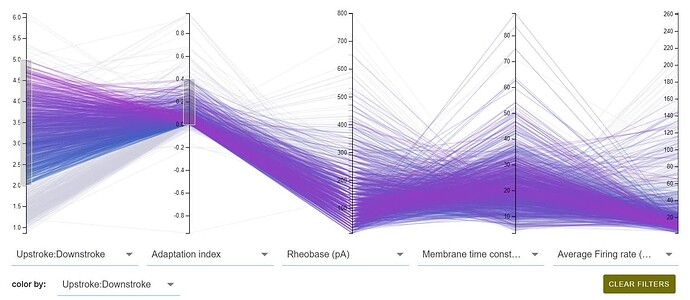
The following table describes the meaning of the properties available in the drop-down manus.For more details on the properties, see the Documentation.
Cell summary cards
The cell summary cards display the results of the selections specified by the filters and the parallel coordinate plot. You can sort the cards according to any cell feature by using the drop-down menus on the top right. For example, the figure below shows cards sorted in ascending value of the Parent:Daughter cell feature.
Each card provides a short summary of cell properties as well as links to pages with detailed information on the electrophysiology data and, when available, the morphology data.
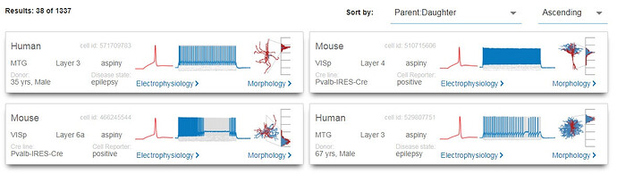
The cards display the following information. For more details on the properties, see the Documentation.
The scale on the right represents the normalized cortical depth, from white matter to pia. The histogram shows the density of neuronal processes as a function of depth.|
|Morphology link|Like to page displaying morphology properties of the cell when they are available.|
Electrophysiology details page
The electrophysiology details page gives you access to the available electrophysiology information for a given cell. The top section of the page provides a summary of the cell properties, while the second allows you view the traces recorded for different stimulus types. For details on the experimental methods, see the Documentation.
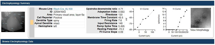
The following discussion explains how to use the different menus and controls on the page to view and download the electrophysiology data. If neuronal models are available for that cell, you can choose to view the simulated data on the page and also download the model parameters. See also the Data access and download section.
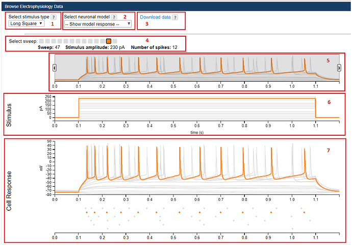
Select Stimulus type: A drop-down menu from which you can select the stimulus type and see the resulting Cell Response.
- Select Neuronal Model: When available, neuronal models have been run on the data and when selected will open below the recorded Cell Response.
- Download Data: This link will download the .nwb file with the data from this experiment. For more information, see [here] FIX (http://ihelp.corp.alleninstitute.org/display/celltypes/API).
- Select Sweep: Select sweeps will be available for you to inspect from this view. As you hover your mouse over each colored square, not only do you see the resulting graphs change to reflect the sweep selected, but you also will see sweep metadata (Sweep #, Stimulus amplitide ¶ and # of spikes) listed below the squares. Once you click on a colored square, you can use left/right arrow keys to move between the sweeps.
- Slider Bar: This feature allows you to zoom in and out of the Stimulus, Cell Response and Model views by clicking and dragging on the arrows.
- Stimulus: The stimulus injected into the cell.
- Cell Response: The response of the cell to the injected stimulus.
Stimulus Types
Different sets of stimulation waveforms were used in order to:
- Interrogate intrinsic membrane mechanisms that underlie the input/output function of neurons
a. Linear and non-linear subthreshold properties
b. Action potential initiation and propagation
c. Afterhyperpolarization/afterdepolarization - Understand aspects of neural response properties in vivo
a. Stimulation frequency dependence (theta vs. gamma) of spike initiation mechanisms
b. Ion channel states due to different resting potentials in vivo - Construct and test computational models of varying complexity emulating the neural response to stereotyped stimuli
a. Generalized leaky-integrate-and-fire (GLIF) models
b. Biophysically and morphologically realistic conductance-based compartmental models


Morphology details page
The morphology details page gives you access to the available morphology information for a given cell. The top section of the page provides a summary of the cell properties, while the second displays two orthogonal projections of the biocytin filled neuron and the neuron’s 3D morphology reconstruction. From this page, you can also view the stack of high resolution images used for the reconstruction. For details on the imaging and neuron reconstruction methods, see the Documentation.

The following discussion explains how to use the different menus and controls on the page to view and download the morphology data. See also the Data access and download section.

From the Projected top view, you can zoom into the picture from the on-screen navigation tools, the Keyboard Commands or using your scroll wheel. The two views of the neuron are synched so zooming in on one will also zoom the other. Clicking on “View image stack” will take you to an image viewer to view the individual images taken of this neuron.
The image viewer of the 3D neuron reconstruction allows for visualization of the reconstructed neuron using the onscreen navigation tools. Clicking “Reset” will reset the neuron to its default view. The legend in the 3D reconstruction indicates the various components of the reconstruction.
You can download both the reconstruction (as an .swc file) or the calculated morphology measurements (as an XML) from the links below the viewers.
Morphology Image Stack
Clicking “View Image Stack” while browsing the Morphology data will take you to our image viewer. The title bar includes the Mouse Line, the Specimen ID, the structure and the hemisphere. The “Configure” icon opens a menu that will allow you to vary the image contrast and download the individual images. The entire image stack can be navigated through using the on screen navigation tools, using the Keyboard Commands or by clicking on the Projected Side View.
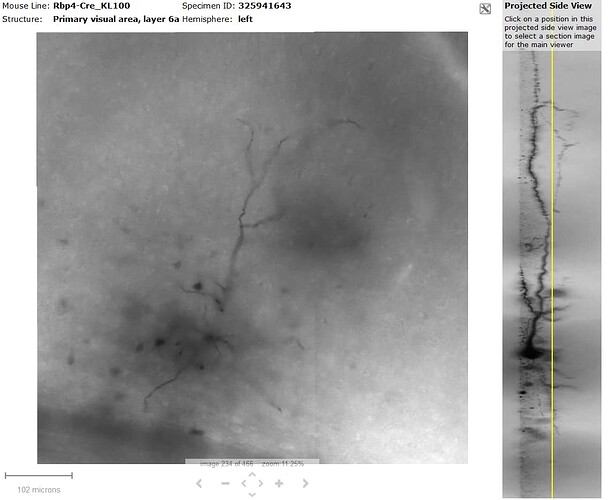
Scale Bar
Shows the current viewing resolution of the image, in microns. This value dynamically changes as you zoom in/out of the image. You can position the scale bar anywhere on the main image by dragging the scale bar by its ruler.
You can toggle the orientation of the scale bar from horizontal to vertical by clicking on the scale bar text.
Keyboard Commands
Neuronal models
Reprocessing of the data occurred for the March 2016 release so any analysis performed prior to the March 2016 release date should be performed again with the new models.
The Allen Cell Types Database contains three types of neuronal models: two biophysical models and generalized leaky integrate-and-fire (GLIF) models. These models attempt to mathematically reproduce a cell’s recorded response to a current injection. The biophysical models take into account dendritic morphological structure, whereas GLIF models are simple point neuron models that represent the neuron as a single compartment.
There are five levels of GLIF models with increasing levels of complexity. The most basic model is a simple leaky integrate-and-fire equation. More advanced GLIFs attempt to model variable spike threshold, afterspike currents, and threshold adaptation.
For more detailed information on each of the models, see the Documentation.
Data access and download
As indicated above, you can download electrophysiology recordings, morphology image data, 3D reconstructions and neuronal model parameters using links in the electrophysiology and morphology details pages for a cell.
You can also access the data programatically and obtain sample code to run your own model simulations. For more details go to the Download page.
Learn about API For Allen Developing Mouse Brain Atlas with comprehensive guides and examples from Allen Institute for Brain Science.
The Allen Developing Mouse Brain Atlas provides in situ hybridization (ISH) image data for approximately 2,000 genes over embryonic and postnatal timepoints. Each data set is processed through an informatics analysis pipeline to obtain spatially mapped quantified expression information.
From the API, you can:
Download images
Download quantified expression values by structure

Download quantified expression values as 3-D grids
Query the correlative search service

Query the image synchronization service

Download atlas images, drawings and structure ontology
This document provides a brief overview of the data, database organization and example queries. API database object names are in camel case. See the main API documentation for more information on data models and query syntax.
Experimental Overview and Metadata
Experimental data from this atlas is associated with the “Developing Mouse Brain” Product.
Multiple genes were assayed using each Specimen. Typically, the sectioning scheme divided each brain into 4 to 8 interleaving SectionDataSets depending on the age of the specimen.
Section thickness is 20 micron for the earlier timepoints up to P4 and 25 micron for P14 and older. Section thickness is an attribute of the SectionDataSet object.
Image resolution is variable (0.99 - 1.049 microns) and is reported as an attribute of SectionImage.
Each gene was assayed with one sagittal SectionDataSet at each of the 7 main developmental timepoints (E11.5, E13.5, E15.5, E18.5, P4, P14, P28). A subset of genes also has coronal SectionDataSets, replicate sagittal experiments and/or data for intermediate and aging timepoints.
To support the generation of structure/age summaries for the web application, one sagittal SectionDataSet is selected as the representative for each age. This is reported as the boolean delegate attribute of SectionDataSet.
From the API, detailed information about Genes, Probes, SectionDataSets and SectionImages can be obtained using RMA queries.
Examples
http://api.brain-map.org/api/v2/data/Gene/query.xml?criteria=products[id$eq3]
- All experiments associated with gene netrin G1 (Ntng1)
http://api.brain-map.org/api/v2/data/SectionDataSet/query.xml?criteria=[failed$eqfalse],products[id$eq3],
genes[acronym$eq'Ntng1']&include=genes,section_images,specimen(donor(age))
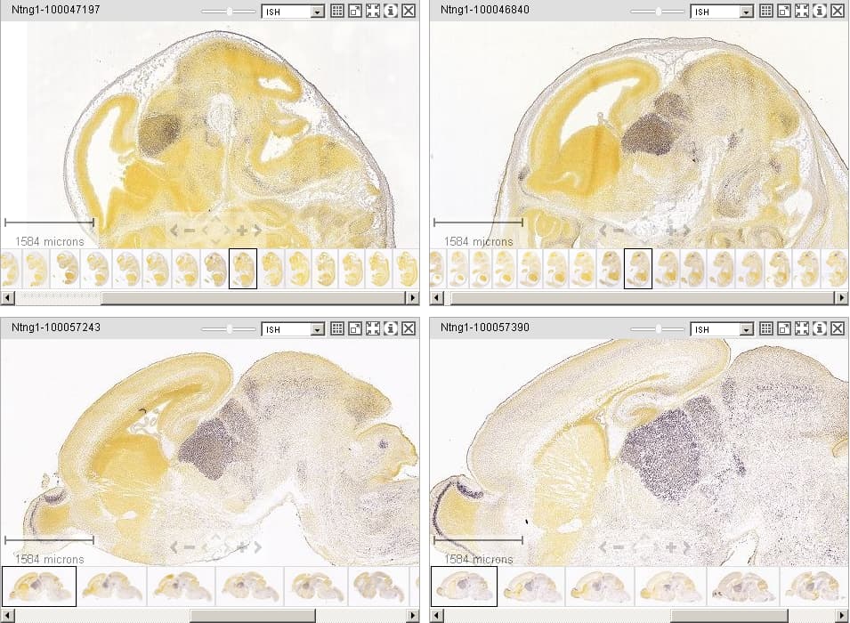
See the image download page to learn how to download images at different resolutions and regions of interest.
Informatics Data Processing
The informatics data processing pipeline produces results that enable the navigation, analysis and visualization. The pipeline consists of the following components:
- a set of age-matched annotated 3-D reference spaces,
- an alignment module,
- an expression detection module,
- an expression gridding module, and
- a structure unionizer module.
The output of the pipeline is quantified expression values at a grid voxel level and at a structure level according to the integrated reference atlas ontology. The grid level data are used downstream to provide a correlative gene search service and to support visualization of spatial relationships. See the informatics processing whitepaper for more details.
3-D Reference Models
The backbone of the automated pipeline is a set of annotated 3-D reference spaces for each of the 7 developmental stages. For each stage, a brain volume was reconstructed from section images from a single specimen. Each 3-D reference space is in PIR orientation (+x = posterior, +y = inferior, +z = right).
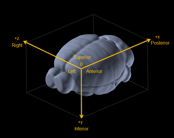
Structural delineation were extracted from the associated 2-D reference atlas plates and interpolated to create 3-D annotations. Structures in the reference atlas are arranged in a hierarchical organization. Each structure has one parent and denotes a “part-of” relationship. Structures are assigned a color to visually emphasize their hierarchical positions in the brain. Note: the structural hierarchy used in this atlas is based on a systematic developmental ontology that differs from the ontology used for processing the Allen Mouse Brain Atlas.
See the atlas drawings and ontologies page for more information.
Three volumetric data files are available for download for each reference space from our download server:
- atlasVolume: uchar (8bit) grayscale Nissl or Feulgen-HP yellow volume of the reconstructed brain.
- annotation: uint (32bit) structural annotation volume matching the atlasVolume. The value represents the ID of the finest level structure annotated for the voxel. Note: the 3-D mask for any structure is composed of all voxels annotated for that structure and all of its descendents in the structure hierarchy.
- gridAnnotation: uint (32bit) structural annotation volume at grid resolution.
All volumetric data is stored in an uncompressed format with a simple text header file in MetaImage format. The raw numerical data is stored as a 1-D array as shown in the figure below.
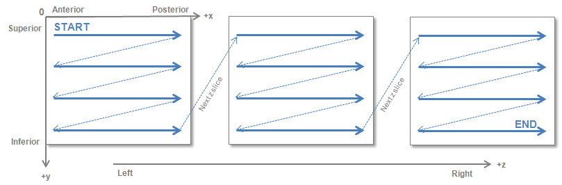
The atlas volume dimension and resolution for each ReferenceSpace vary with age, scanning platform and gene sampling density as listed in the table below.
Table information in CSV format.
The grid dimension and resolution for each ReferenceSpace vary with age and gene sampling density as listed in the table below.
Table information in CSV format.
Example Matlab code snippet to read in the P4 atlas and annotation volume:
% ------------
% Download and unzip the P4 (ReferenceSpace=6) atlasVolume and annotation zip files
% ------------

% atlas volume size
size = [724,403,398];

% VOL = 3-D matrix of atlas Nissl volume
fid = fopen('P4_atlasVolume/atlasVolume.raw', 'r', 'l' );
VOL = fread( fid, prod(size), 'uint8' );
fclose( fid );
VOL = reshape(VOL,size);

% ANO = 3-D matrix of annotation labels
fid = fopen('P4_DevMouse2012_annotation/annotation.raw', 'r', 'l' );
ANO = fread( fid, prod(size), 'uint32' );
fclose( fid );
ANO = reshape(ANO,size);

% Display one coronal section
figure;imagesc(squeeze(VOL(362,:,:)));colormap(gray);
figure;imagesc(squeeze(ANO(362,:,:)));colormap(lines);

% Display one sagittal section
figure;imagesc(squeeze(ANO(:,:,115)));colormap(lines);
figure;imagesc(squeeze(VOL(:,:,115)));colormap(gray);
Example Matlab code snippet to read in the P4 grid annotation volume:
% -----------
% Download and unzip the P4 (ReferenceSpace=6) gridAnnotation zip files
% -----------

%  grid volume size
sizeGrid = [77,43,50];

% ANOGD = 3-D matrix of grid-level annotation labels
fid = fopen( 'P4_DevMouse2012_gridAnnotation/gridAnnotation.raw', 'r', 'l' );
ANOGD = fread( fid, prod(sizeGrid), 'uint32' );
fclose( fid );
ANOGD = reshape(ANOGD,sizeGrid);

% Display one coronal and one sagittal section
figure;imagesc(squeeze(ANOGD(36,:,:)));colormap(lines);
figure;imagesc(squeeze(ANOGD(:,:,14)));colormap(lines);
Image Alignment
The aim of image alignment is to establish a mapping from each SectionDataSet to its exact or closest age matched ReferenceSpace. The reference-space-id attribute indicates which reference space the data has been aligned to. The module reconstructs a 3-D Specimen volume from its constituent SectionImages and registers the volume to the 3-D reference model by maximizing image correlation.
Once registration is achieved, information from the 3-D reference model can be transferred to the reconstructed Specimen and vice versa. The resulting transform information is stored in the database. Each SectionImage has an Alignment2d object that represents the 2-D affine transform between an image pixel position and a location in the Specimen volume. Each SectionDataSet has an Alignment3d object that represents the 3-D affine transform between a location in the Specimen volume and a point in the 3-D reference model. Spatial correspondence between any two SectionDataSets from different Specimens can be established by composing these transforms.
For convenience, a set of “Image Synchronization” API methods is available to find a corresponding position between SectionDataSets, the 3-D reference model and structures. Note that all locations on SectionImages are reported in pixel coordinates and all locations in 3-D ReferenceSpaces are reported in microns. These methods are used by the Web application to provide the image synchronization feature in the multiple image viewer.
To support image synchronization across reference spaces, each space has been co-registered and scaled to every other space using a 12 parameter affine transform, allowing brains of different ages to be roughly compared. The image synchronization API methods automatically perform the cross-space transform when requesting to sync data from different reference spaces.
Examples:
http://api.brain-map.org/api/v2/image_to_image/101121829.xml?x=5752&y=3312§ion_data_set_ids=100057390,100047075,100047197,100046840,100057243,100045273,100045230,71924185,70300595
[type or paste code here](http://api.brain-map.org/api/v2/image_to_atlas/101121829.json?x=5752&y=3312&atlas_id=181276165)


Expression Detection
For every ISH SectionImage, a grayscale mask is generated that identifies pixels corresponding to gene expression. The detection algorithm is based on adaptive thresholding and mathematical morphology.
The expression mask image is the same size and pixel resolution as the primary ISH image and can be downloaded through the image download service.
Expression Gridding
For each SectionDataSet, the Gridding module creates a low resolution 3-D summary of the gene expression and projects the data to its exact or closest age matched ReferenceSpace. Casting all data into a canonical space allows for easy cross-comparison of gene expression data within each stage. The expression data grids can also be viewed directly as 3-D volumes or used for analysis such as correlative searches.
Each image in a SectionDataSet is divided into a grid resolution squares. Grid resolution varies with age ranging from 80 x 80 µm at E11.5 to 200 x 200 µm at P28. Pixel-based gene expression statistics are computed using information from the primary ISH and the expression mask:
- expression density = sum of expressing pixels / sum of all pixels in division
- expression intensity = sum of expressing pixel intensity / sum of expressing pixels
- expression energy = expression intensity * expression density
Each per-image 2-D expression grid is smoothed and rotated to form a 3-D grid. Z-direction smoothing is applied to the 3-D grid which is then transformed into the targeted reference space.
Grid data can be downloaded for each SectionDataSet using the 3-D Expression Grid Data Service. The service returns a zip file containing the volumetric data for expression density, intensity and/or energy in an uncompressed format with a simple text header file in MetaImage format. Structural annotation for each grid voxel can be obtained via the ReferenceSpace gridAnnotation volume file.
Note: Coronal SectionDataSets span both hemispheres while sagittal SectionDataSets only span the left hemisphere. Voxels with no data are assigned a value of “-1”.
Examples:
http://api.brain-map.org/grid_data/download/100054927
http://api.brain-map.org/grid_data/download/100054927?include=intensity,density
The expression data grid can be viewed in the Brain Explorer® 2 desktop program. Each grid voxel is rendered as a colorized sphere where the diameter represents expression energy and the color encodes expression intensity. In addition, a preview of the expression data grid is shown on the Web application as a series of maximum density projection images.
Example Matlab code snippet to read an energy grid volume:
%------------
% Download and unzip the energy grid file for P4 Rora Pdyn SectionDataSet
% -----------

%  grid volume size
sizeGrid = [77,43,50];

% ENERGY = 3-D matrix of expression energy grid volume
fid = fopen('Rora_P4_sagittal_100054927/energy.raw', 'r', 'l' );
ENERGY = fread( fid, prod(sizeGrid), 'float' );
fclose( fid );
ENERGY = reshape(ENERGY,sizeGrid);

% Display one coronal and one sagittal section
figure;imagesc(squeeze(ENERGY(36,:,:)));colormap(gray);
figure;imagesc(squeeze(ENERGY(:,:,14)));colormap(gray);
Structure Unionization
Expression statistics at a structural level are also computed by combining/unionizing grid voxels with the same 3-D structural label. Expression statistics are encapsulated as a StructureUnionize object associated with one Structure and one SectionDataSet. StructureUnionize data is used in the web application to display expression summary colormaps for a set of coarse structures over development.
Expression statistics are encapsulated as a StructureUnionize object associated with one Structure and one SectionDataSet and can be downloaded via RMA.
StructureUnionize data is used in the web application to generate an expression summary heatmap for a set of coarse structures over the 7 main developmental timepoints assayed.
Example:
- Fetch expression energy values for the delegate SectionDataSet at each of the 7 developmental ages for coarse-level structures RSP, Tel, PedHy, p3, p2, p1, M, PPH, PH, PMH and MH in CSV format
http://api.brain-map.org/api/v2/data/query.csv?criteria=model::StructureUnionize,rma::criteria,section_data_set[delegate$eqfalse] (genes[id$eq21177],specimen(donor(age[name$in'E11.5','E13.5','E15.5','E18.5','P4','P14','P28']))),
structure(structure_sets_structures(structure_set[name$eq'Developing Mouse - Coarse']))
&order=ages.embryonic$desc,ages.days,structures.graph_order&num_rows=100
&tabular=structure_unionizes.section_data_set_id,ages.name as age,ages.embryonic,ages.days,
structures.acronym,structures.name,structures.graph_order,structure_unionizes.expression_energy
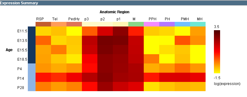
Expression Grid Search Service
A expression grid service has been implemented to allow users to instantly perform a correlation search over the ~2,000 genes to find genes that have a similar spatio-temporal profile to a seed gene.
The expression grid search service is available through both the Web application and API.
To perform a Correlation search, a user selects a seed Gene, a spatial domain and a set of timepoints over which the similarity comparison is to be made. All voxels belonging to any of the domain structures and specified timepoints form the domain voxel set. Pearson’s correlation coefficient is computed between the domain voxel set from the seed Gene and every other Gene in the Product. The return list is sorted by descending correlation coefficient.
Note: Only the 7 main developmental timepoints (E11.5, E13.5, E15.5, E18.5, P4, P14, P28) can be used as temporal domain. For each timepoint, the delegate SectionDataSet is used in the computation.
See the connected service page for definitions of service::dev_mouse_correlation parameters.
Example:
- Correlation search for genes with similar expression to Neurod1 within the telencephalic vesicle (Tel) at age P4
http://api.brain-map.org/api/v2/data/query.xml?criteria=service::dev_mouse_correlation[row$eq17779] [structures$eq'Tel'][ages$eq'P4']
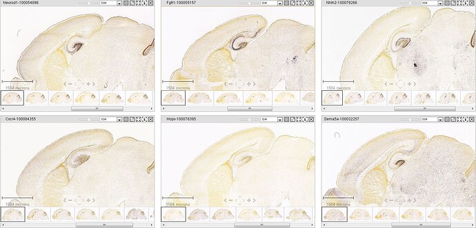
Figure: Screenshot of top returns of a correlation search for genes with similar expression as Neurod1 within the telencephalic telencephalic vesicle at age P4.
Example:
- Correlation search for genes with similar expression to Neurod1 within Tel over multiple ages P4, P14, P28
http://api.brain-map.org/api/v2/data/query.xml?criteria=service::dev_mouse_correlation[row$eq17779] [structures$eq'Tel'][ages$eq'P4','P14','P28']
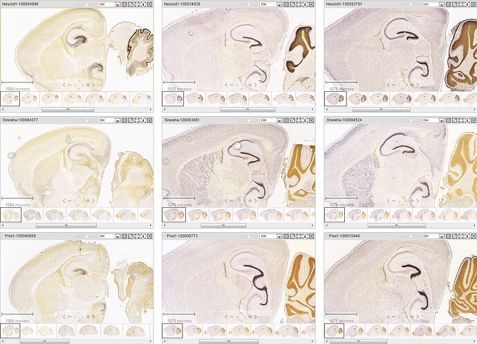
Example:
- Correlation search for genes with similar expression to Nr5a1 over the whole neural plate (NP) and across all 7 ages
http://api.brain-map.org/api/v2/data/query.xml?criteria=service::dev_mouse_correlation[row$eq26171][structures$eq'NP']
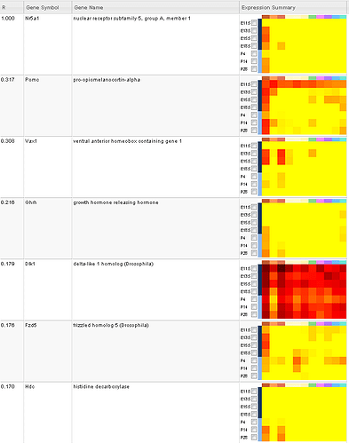
Expert Manual Annotation
ISH data for ages E11.5, E13.5, E15.5 and E18.5 were manually annotated to provide accurate gene expression characteristics for fine level structures. For each SectionDataSet and Structure, gene expression is scored with intensity (Undetected, Low, Medium, High), density (Undetected, Low, Medium, High) and pattern (Undetected, Full, Regional, Gradient) attributes.
Manual annotation results can be accessed through RMA and can be used to search data.
Note: the structural hierarchy associated with the manual annotation differs from the Ontology used for informatics processing of the ISH data.
Examples:
- Download manual annotation for gene Tcf7l2 at E11.5
http://api.brain-map.org/api/v2/data/query.xml?criteria=model::ManualAnnotation,rma::criteria,[section_data_set_id$eq100045897], rma::include,structure,rma::options[order$eq'structures.graph_order$asc']
- Search for E13.5 SectionDataSets with high intensity, regional expression in the diencephalon
http://api.brain-map.org/api/v2/annotated_section_data_sets.xml?structures=112765096 &intensity_values='High'&pattern_values='Regional'&age_names='E13.5'
http://api.brain-map.org/api/v2/structure_graph_download/112755225.json
Learn about Developmental Anatomic Gene Expression Atlas AGEA with comprehensive guides and examples from Allen Institute for Brain Science.
AGEA is an interactive relational atlas based on spatial correlations of gene expression data for ~2000 genes in the Allen Developing Mouse Brain Atlas.
AGEA for the Developing Mouse Brain is used to understand how voxels of the brain are related by gene expression (Correlation), and to find genes expressed at a particular voxel (Gene Finder). Click on the AGEA tab to get started.
Correlation Mode

In correlation mode, use the seed selector to select a starting age by clicking on your age of interest. The next three columns will show you the age you selected flanked by the nearest developmental ages. Also shown in the column headers are the structure and location of the selected voxel and the Pearson’s correlations (please see Informatics whitepaper available from the Documentation tab).
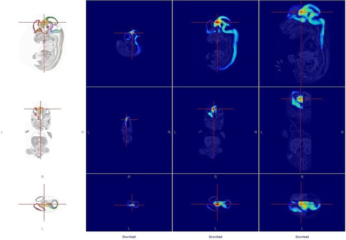
Select a “seed” voxel using the cross hairs in the left hand column from one of the planes of view. The three columns to the right show correlation maps of how other voxels are related to the seed voxel based upon the gene expression of approximately 2000 genes.
Seed Selector
To begin, select an age from the upper left hand corner. Maps of the age-appropriate reference space are shown in sagittal, coronal and horizontal planes in the left-most column. Navigate by clicking on a spot in one plane of view; this will appropriately adjust the other planes of view. Click on the maps to position the red crosshairs on the voxel of interest. Maps are only available for one brain hemisphere, shown by the overlay of reference atlas colors on the Nissl reference space.
Correlation Maps
The correlation maps are shown as heat maps (red is the highest correlation to the seed voxel) with one column for each age. The age chosen with the seed selector is shown, as well as the next youngest and the next oldest ages.
Gene Finder
Once a seed is selected and correlation maps are shown, you can retrieve a list of genes enriched in the region correlated to the seed voxel.

First, click on the “Gene Finder” tab. Then, click on “Find Genes” for the particular age you are interested in.
Search Results
Using the Gene Finder function in AGEA will return a list of genes that fit your search criteria. Searching for genes at an age other than the age chosen in the seed selector will return a list of genes that fit both ages.

Each column includes:
| Column | Description |
|---|---|
 | Allows you to select one or more experiments to view by clicking “View Selections” |
| Fold Change | Fold change of the gene expression in the selected voxel over the thresholded voxels |
| Gene Symbol | Clicking on this link will take you to the Gene Detail page |
| Gene Name | Clicking on this name will seed the right panel with the 3-D thumbnail images of this experiment, and allow you to search for other similar genes from the Correlation Search box |
| Seed Location | A representative image from the age selected in the Seed Selector |
| Map Location | (If two ages were selected) A representative image from the age selected with Gene Finder |
Please refer to the Informatics Data Processing white paper available from the Documentation tab for additional details.
Learn about Allen Developing Mouse Brain Atlas In Situ Hybridization ISH Data with comprehensive guides and examples from Allen Institute for Brain Science.
Viewing Gene Expression Data
The Allen Developing Mouse Brain Atlas offers colorimetric In Situ Hybridization data at cellular resolution at seven stages of mouse development. Choose among the following options for retrieving the data:
- Search from the tag cloud by Gene Classification
- Use Gene Search to locate genes’ data by name, symbol, NCBI accession number, or Entrez Gene ID.
- You can also use Gene Search with Boolean operators on specific field names using Boolean Syntax Query.
- Search for manually curated enhanced gene expression data using the Annotation Search.
- Search for genes with enhanced expression by anatomic region using Anatomic Search.
- Search for genes with enhanced expression by developmental stage using Temporal Search.
- Explore related studies using the Extended Studies radio button.

Gene Search
To search for a specific gene by name, symbol, NCBI accession number, or Entrez gene ID, type your query into the text box, making sure the “Gene Search” radio button is selected. As you type, genes that match your search string will be suggested to you. Select an item from the list and click the “Search” button. The results are displayed in a list that shows all genes with expression data that match your query.
Tips for searching:
- If you are unsure of spelling, begin typing the gene identifier and suggestions will be offered.
- Press the ‘Enter’ key instead of clicking the “Search” button.
- Select the “Show exact matches only” check box to remove the implied wildcards. This is useful if you want to return only those genes that exactly match your search text.
- Place the search text within quotes to include spaces or special characters.
- When searching for more than one gene, separate each search term by a comma.
Boolean Syntax Query
The following special operators can be used to build queries:
- The AND function is implicit, so spaces between words that are not separated by an operator will be treated like AND.
- OR has higher operator precedence than AND.
- Parentheses can be used to group criteria, but nested parentheses are not supported at this time.
Annotation Search
While our automatically-generated semi-quantitative analysis tools (Anatomic Search and Temporal Search) provide an informative global view of gene expression in the developing brain, these tools provide gene expression information primarily about larger brain regions, with limited resolution for precise brain areas. The Annotation Search feature utilizes expert-guided manual annotation performed by Dr. Salvador Martinez of the Neurosciences Institute, Miguel Hernandez University and CSIC in Alicante, Spain.
This feature allows you to search the annotation data for all genes that match specific gene expression criteria. Start by selecting a structure from the developing mouse ontology and then indicate the age(s), the expression intensity(ies), the expression density(ies) and the expression pattern(s). To understand the criteria used to make these manual annotations, please see the Annotation whitepaper in the Documentation tab.

To look for genes that also match additional criteria, click the “+” button to add another row to your search. Remove extra rows by clicking the “x” box. Once you have entered your search criteria, click on the “Search” button. The results are displayed as a list of genes demonstrating gene expression patterns that match your query.
Any genes that meet the criteria in ALL rows of the search will be returned. If two or more specific ages (or intensities, densities or patterns) are selected in a single row, the search will find all results that match any one of the criteria (i.e. an “OR” search).
For example, this query displayed above will return many results because the second line specifies that either the E15.5 or E18.5 timepoints can have high expression in the prepontine hindbrain. The query displayed below looks similar but it is much more selective; only a few genes have high expression in PPH for E15.5 AND E18.5, AND Low expression in E13.5.
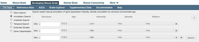
Viewing Annotation Search Results
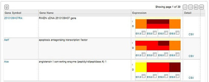
Search returns include a list of experiments that fulfill your search criteria listing the gene symbol, the gene name, an expression summary illustrated in a heatmap format and a link to the .csv annotation document for that gene. The expression summary will include:
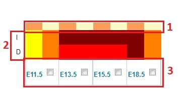
- Structures - The structures you selected colored according to the reference atlas colors as column headers in the heatmap.
- Annotation Results - Row headers are the Intensity (I) and the Density (D) and colored as follows: Grey - Cannot Annotate, Yellow - Undetected, Orange - Low, Red - Medium, Burgundy - High.
- Stages for each experiment - Click on the check boxes to view image series in a separate window.

Anatomic Search

Select the “Anatomic Search” radio button to search for genes that are predominantly enriched within the selected brain structure. Results will be returned for the specified age. Experiments are ranked by the specificity of the gene in the brain structure of interest as opposed to adjacent brain regions. The rank is defined as the ratio of sum of expressing pixel intensities in the numerator set (target region) over the sum of expressing pixel intensities in the denominator set (a defined set of non-overlapping structures, see Data Processing Whitepaper under the Documentation tab). Thirteen structures are generally available for search for each age, with the exception of E11.5, for which five structures are available. The results are provided as a list of experiments for the given age and search query.
Please refer to the Informatics Data Processing white paper in the Documentation tab for additional details.
Temporal Search
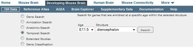
Select the “Temporal Search” radio button to search for genes that are enriched at a specific age within the selected structure. Note that this feature does not search for spatial enrichment; Anatomic Search should be used for that purpose. This search feature compares gene expression in the given structure at the given age and compares it to expression in the same structure at 7 other time points. Results are returned as a list of experiments ranked by their temporal enrichment in descending order, with the most temporally enriched genes first.
Please refer to the Informatics Data Processing white paper in the Documentation tab for additional details.
Correlation Search
Once you have found a gene of interest, you can also find genes with a similar expression profile to your gene of interest using the Correlation Search option: once a gene is selected by clicking on the gene name, from the right-hand panel, choose one or more structures from the structure drop-down menu and one or more ages from the ages drop-down menu and then click “Search”. Your search will result in a list of genes with a similar expression pattern to your search criteria.

Extended Studies
A select group of genes were sampled deeper and can be viewed using the Extended Studies radio button.
High Temporal Sampling Study
Select “High Temporal Sampling Study” to see ~20 developmental marker genes characterized by ISH in coronal plane with higher temporal resolution, including 8 embryonic developmental stages and 6 early postnatal stages.
Aging Study
Select “Aging Study” to see ~300 genes surveyed in aged brain at 18 and 24 months.
Viewing Search Results
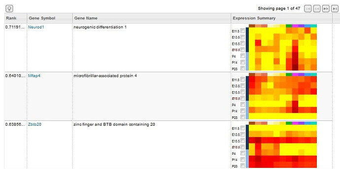
Searches will return a list of genes based on the input search criteria. Each row includes the following information.
Select the experiments to view in greater detail by clicking the checkboxes next to gene and age of interest. Experiments will be saved in your cache until you select the “Clear Selections” button at the bottom of the page. After selecting one or more experiments, click the “View Selections” button.
Once you have selected a gene (by clicking on it’s Gene Name), you can view the rotating 3-D thumbnails in the right hand panel and you can look for genes with a similar expression profile.
Experiment Image Viewer
The experiment image viewer displays images for each selected experiment in a Zoom and Pan viewer. This viewer makes it easy to compare experiments with each other and with the Reference Atlas.
Multiple image series can be opened on the same page to enable side-by-side comparisons. Arrange the experiments by dragging a viewer by the title bar and dropping in a new location. Add one or more reference atlases by selecting from the “Atlases” drop-down menu in the upper-right hand corner of the window.
If you are viewing more than one experiment, open the configuration options to change the number of columns displayed in the window. The configuration options are accessible by clicking on the button with a “gear” icon to the right of the “Atlases” menu.
The gene symbol is displayed in the title bar along with the Allen Institute image series ID. Additional details are displayed across the top of the viewing area, including the image index, tissue index, and tissue location.
Thumbnails for the entire image series are displayed across the bottom of the viewer in section order. Click a thumbnail to select it for viewing, or use the keyboard to navigate through the set. The current selection is outlined in black.
Gene Detail
When you click on the gene symbol, you will be taken to a page that describes the experiments involving this gene in detail. The data returned includes gene detail metadata, the Expression Summary and a list of the experiments performed.
Gene detail metadata includes the name of the gene, any aliases this gene may have, the organism that the experiment was conducted on, the Entre ID and the chromosome location of the gene.

The gene expression summary is represented in heatmap format with the age of the mouse on the vertical axis and the anatomic region on the horizontal axis color-coded to the reference atlas. The heatmap illustrates increasing expression energy ranging from a log value of -1.5 in the yellow to 3.5 in the dark red.
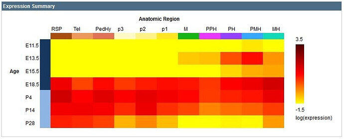
A list of experiments conducted on this gene includes:
| Column | Description |
|---|---|
| Click this box to view experiment(s) in the interactive viewing tool |
| Experimental Detail | Click on this link to be taken to the Experimental Detail page |
| Developmental Stage | Indicates both the developmental age and the Theiler Stage |
| Example Image | Shows a single image from the experiment |
| Rotating Thumbnails | Shows a 3-D image of the gene expression that can be rotated using the slider bar in the column header |
| 3-D File | Links to open up the individual experiment in the Brain Explorer 3-D software. Clicking on the column header will open all the experiments in the Brain Explorer |

Click on one or more experiments to view all the experiments in an interactive environment. This data can also be downloaded as an XML query by clicking on the “This data is also available as XML” link.
Experimental Detail
When the experiment is selected by clicking on the experimental ID link, a summary of the experimental detail is returned. The data includes 1) Experiment and Specimen metadata and a link to Related Institute Data 2) an interactive 3-dimensional representation of gene expression, 3) an interactive image viewer that displays the images in the experiment 4) a histogram of the expression energy in 11 different structures, and 5) Probe metadata including forward and reverse primers and probe sequence.
Hovering your mouse over the histogram will sync the image in the single image viewer with the section corresponding to that structure and expression.
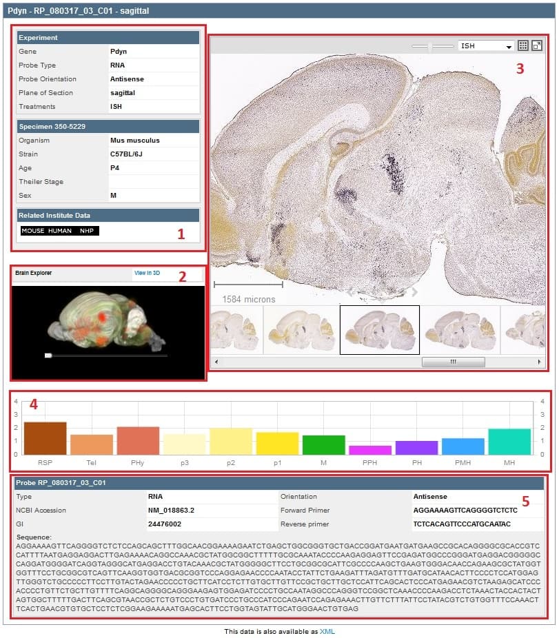
Using the Zoom and Pan (ZAP) Image Viewer
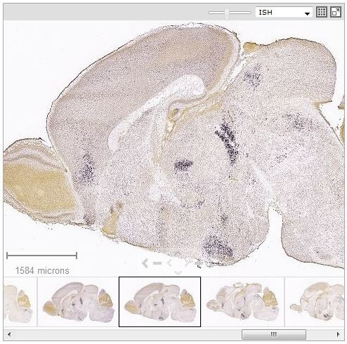
The Zoom and Pan (ZAP) Image Viewer is a powerful tool to navigate and view the images in an experiment. The main part of the viewer is an interactive window where an image can be repositioned by dragging with a mouse. Use the scroll wheel, the on screen navigation tools or the keyboard to zoom in or out.
Select other images in the experiment by clicking on a thumbnail image below the main viewer.
Scale Bar
Drag the scale bar with your mouse to the desired location. Click the text with your mouse to toggle between horizontal and vertical.
Using the ZAP Viewer Toolbar
Use the toolbar to take actions on the image that currently has focus. Toolbar controls include:
| Control | Function |
|---|---|
 | Move the slider bar to the left to intensify the contrast or color |
 | Select ISH, Nissl or Expression image type |
 | Display all thumbnail images in a single ‘contact sheet’ |
 | Open the selected image in the image viewer tool |
 | Synchronize all other Zap viewers on the page that support synchronization to the currently selected image |
 | Open a new browser window to review metadata for the image series |
 | Close the Zap viewer |
Keyboard Commands
Use the keyboard to navigate through the image series and synchronize the viewers on the page. Keyboard commands include:
You can also use the arrow keys to pan the current image.
Expression Energy
The expression mask image display highlights those cells that have the highest probability of gene expression using a heat map color scale (from low/blue to high/red).
The Expression Energy was calculated as follows: Within a given area A (voxel or structure), expression energy = (sum of intensity of expressing pixels in A) / (sum of all pixels in A)
Using the High Resolution Image Viewer
The image viewer enables you to view a high resolution image in its own re-sizable window. It is possible to open multiple images by opening multiple windows.
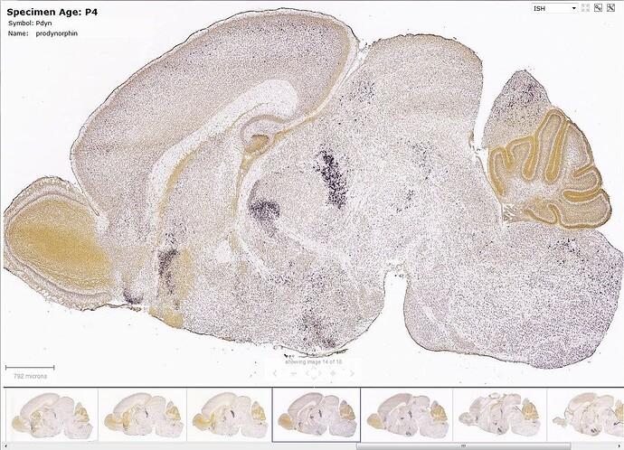
Interacting with the High Resolution Image Viewer is similar to using the ZAP Viewer with some enhanced features accessible from icons in the top right hand of the main image viewer.
| Icon | Description |
|---|---|
 | View ISH, Expression Energy, or Reference Stain (Nissl or Feulgen-HP Yellow) |
 | View experiment side by side with the Interactive Atlas Viewer |
 | Allows you to access setting options, including downloading the current image |
Learn about API For Mouse Brain Atlas with comprehensive guides and examples from Allen Institute for Brain Science.
The Allen Mouse Brain Atlas provides genome-wide in situ hybridization (ISH) image data for approximately 20,000 genes in adult mice. Each data set is processed through an informatics analysis pipeline to obtain spatially mapped quantified expression information.
From the API, you can:
- Download images
- Download quantified expression values by structure
- Download quantified expression values as 3-D grids
- Query the differential and correlative search services
- Query the image synchronization service
- Download atlas images, drawings and structure ontology
This document provides a brief overview of the data, database organization and example queries. API database object names are in camel case. See the main API documentation for more information on data models and query syntax.
Experimental Overview And Metadata
Experimental data from this atlas is associated with the “Mouse Brain” Product.
Multiple genes were assayed using each Specimen. Typically, the sectioning scheme divided each brain into eight interleaving SectionDataSets with 200 µm sampling density (= 8 x 25 µm thickness).
Each gene was assayed with at least one sagittal SectionDataSet. A subset of genes also has a coronal SectionDataSet and/or replicate experiments. A sagittal SectionDataSet spans the left hemisphere starting with the most lateral section located at where the hippocampus starts to appear to just past the midline yielding ~20 SectionImages at 200 µm sampling density. A coronal SectionDataSet spans both hemispheres starting with the most posterior section showing the cerebellum and hindbrain to the most anterior section showing the olfactory bulb, yielding ~60 SectionImages at 200 µm sampling density. The left side of a coronal SectionImage corresponds to the left hemisphere.
A manual QC protocol defines the criteria for failing experiments due to production issues, discarding damaged SectionImages, verifying and adjusting the tissue bounding boxes, as well as for identifying “dark” artifacts such as bubbles and tears.
From the API, detailed information about Genes, Probes, SectionDataSets and SectionImages can be obtained using RMA queries.
Examples
From the above query, gene Pdyn has one sagittal SectionDataSet (id=69782969) and one coronal SectionDataSet (id=71717084). In the web application, images from the experiment are visualized in an experiment detail page. All displayed information, images and structural expression values are also available through the API.
See the image download page to learn how to download images at different resolutions and regions of interest.

Informatics Data Processing
The informatics data processing pipeline produces results that enable the navigation, analysis and visualization. The pipeline consists of the following components:
- an annotated 3-D reference space,
- an alignment module,
- an expression detection module,
- an expression gridding module, and
- a structure unionizer module.
The output of the pipeline is quantified expression values at a grid voxel level and at a structure level according to the integrated reference atlas ontology. The grid level data are used downstream to provide a differential and correlative gene search service and to support visualization of spatial relationships. See the informatics processing whitepaper for more details.
3-D Reference Models
The backbone of the automated pipeline is an annotated 3-D reference space based on the same Specimen used for the coronal plates of the integrated reference atlas. A brain volume was reconstructed from the SectionImages using a combination of high frequency section-to-section histology registration with low-frequency histology to (ex-cranio) MRI registration. This first-stage reconstructed volume was then aligned with a sagittally sectioned Specimen. Once a straight mid-sagittal plane was achieved, a synthetic symmetric space was created by reflecting one hemisphere to the other side of the volume.
Over 800 Structures were extracted from the 2-D coronal reference atlas plates and interpolated to create symmetric 3-D annotations. Structures in the reference atlas are arranged in a hierarchical organization. Each structure has one parent and denotes a “part-of” relationship. Structures are assigned a color to visually emphasize their hierarchical positions in the brain.
In the May 2015 data release, we introduced a next generation common coordinate framework (CCF v3) based on a population average to support the integration of new mouse brain datasets in the Allen Brain Atlas Data Portal. See the Allen Mouse Common Coordinate Framework whitepaper for detailed construction information.
The Nissl volume and 3-D annotation from the Allen Reference Atlas were deformably registered to the new common coordinate framework to support potential cross-modality analysis of gene expression with new data modalities as they become available in the Data Portal.
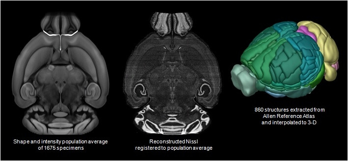
See the atlas drawings and ontologies page for more information.
All coronal data is registered to ReferenceSpace id = 9. All sagittal data is registered to ReferenceSpace id = 10.
ReferenceSpace id = 9 is in PIR orientation (+x = posterior, +y = inferior, +z = right). ReferenceSpace id = 10 is identical to ReferenceSpace id = 9. The reason for the two spaces is to allow left hemisphere sagittal data to correspond to the right hemisphere coronal reference atlas. This is implemented as a z-axis flip transform between the two reference spaces for the purposes of image synchronization (see below).
NOTE: 3-D annotation volumes were updated in the May 2015 release to reflect the introduction of the next generation of the Allen Mouse Common Coordinate Framework (CCFv3). Annotation volumes from the October 2014 release (mapped to CCFv2) can be access through our data download server (see instructions).
Three volumetric data files are available for download:
- atlasVolume : uchar (8bit) grayscale Nissl volume of the reconstructed brain at 25 µm resolution.
- annotation : uint (32bit) structural annotation volume at 25 µm resolution. The value represents the ID of the finest level structure annotated for the voxel. Note: the 3-D mask for any structure is composed of all voxels annotated for that structure and all of its descendents in the structure hierarchy.
- gridAnnotation : uint (32bit) structural annotation volume at grid (200 µm) resolution for gene expression analysis.
All volumetric data is stored in an uncompressed format with a simple text header file in MetaImage format. The raw numerical data is stored as a 1-D array as shown in the figure below.
Example Matlab code snippet to read in the 25µm atlas and annotation volume:
% Download and unzip the atlasVolume and annotation zip files

% 25 micron volume size

size = [528 320 456];

% VOL = 3-D matrix of atlas Nissl volume

fid = fopen('atlasVolume/atlasVolume.raw', 'r', 'l' );

VOL = fread( fid, prod(size), 'uint8' );

fclose( fid );

VOL = reshape(VOL,size);

% ANO = 3-D matrix of annotation labels

fid = fopen('annotation.raw', 'r', 'l' );

ANO = fread( fid, prod(size), 'uint32' );

fclose( fid );

ANO = reshape(ANO,size);

% Display one coronal section

figure;imagesc(squeeze(VOL(264,:,:)));colormap(gray);

figure;imagesc(squeeze(ANO(264,:,:)));colormap(lines);

% Display one sagittal section

figure;imagesc(squeeze(ANO(:,:,220)));colormap(lines);

figure;imagesc(squeeze(VOL(:,:,220)));colormap(gray);
Example Matlab code snippet to read in the 200µm atlas and annotation volume:
% Download and unzip the gridAnnotation zip files

% 200 micron volume size

sizeGrid = [67 41 58];

% ANOGD = 3-D matrix of grid-level annotation labels

fid = fopen( 'gridAnnotation.raw', 'r', 'l' );

ANOGD = fread( fid, prod(sizeGrid), 'uint32' );

fclose( fid );

ANOGD = reshape(ANOGD,sizeGrid);

% Display one coronal and one sagittal section

figure;imagesc(squeeze(ANOGD(34,:,:)));colormap(lines);

figure;imagesc(squeeze(ANOGD(:,:,28)));colormap(lines);
Image Alignment
The aim of image alignment is to establish a mapping from each SectionImage to the 3-D reference space. The module reconstructs a 3-D Specimen volume from its constituent SectionImages and registers the volume to the 3-D reference model by maximizing image correlation.
Once registration is achieved, information from the 3-D reference model can be transferred to the reconstructed Specimen and vice versa. The resulting transform information is stored in the database. Each SectionImage has an Alignment2d object that represents the 2-D affine transform between an image pixel position and a location in the Specimen volume. Each SectionDataSet has an Alignment3d object that represents the 3-D affine transform between a location in the Specimen volume and a point in the 3-D reference model. Spatial correspondence between any two SectionDataSets from different Specimens can be established by composing these transforms.
For convenience, a set of “Image Sync” API methods is available to find corresponding position between SectionDataSets, the 3-D reference model and structures. Note that all locations on SectionImages are reported in pixel coordinates and all locations in 3-D ReferenceSpaces are reported in microns. These methods are used by the Web application to provide the image synchronization feature in the multiple image viewer (see Figure).
Examples:
- Fetch alignment transforms parameters for the sagittal Pdyn SectionDataSet
- Sync a location between the sagittal and coronal Pdyn SectionDataSets
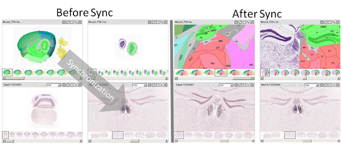
Expression Detection
For every ISH SectionImage, a grayscale mask is generated that identifies pixels corresponding to gene expression. The detection algorithm is based on adaptive thresholding and mathematical morphology.
The expression mask image is the same size and pixel resolution as the primary ISH image and can be downloaded through the image download service.
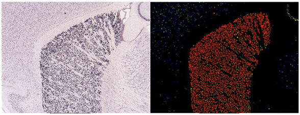
Expression Gridding
For each SectionDataSet, the Gridding module creates a low resolution 3-D summary of the gene expression and projects the data to the common coordinate space of the 3-D reference model. Casting all data into a canonical space allows for easy cross-comparison of gene expression data from every Product. The expression data grids can also be viewed directly as 3-D volumes or used for analysis (i.e. differential and correlative searches).
Each image in a SectionDataSet is divided into a 200 x 200 µm grid. Pixel-based gene expression statistics are computed using information from the primary ISH and the expression mask:
- expression density = sum of expressing pixels / sum of all pixels in division
- expression intensity = sum of expressing pixel intensity / sum of expressing pixels
- expression energy = expression intensity * expression density
Each per-image 2-D expression grid is smoothed and rotated to form a 3-D grid. Z-direction smoothing is applied to the 3-D grid which is then transformed into the standard reference space.
Grid data can be downloaded for each SectionDataSet using the 3-D Expression Grid Data Service. The service returns a zip file containing the volumetric data for expression density, intensity and/or energy in an uncompressed format with a simple text header file in MetaImage format. Structural annotation for each grid voxel can be obtained via the ReferenceSpace gridAnnotation volume file.
Note: while the reference space spans both hemispheres, sagittal SectionDataSets only span the left hemisphere. Voxels with no data are assigned a value of “-1”.
Examples:
- Download expression energy grid file for the coronal Pdyn SectionDataSet
- Download expression density and intensity grid files for the same SectionDataSet
NOTE: Grid data were updated in the May 2015 release to reflect the introduction of the next generation of the Allen Mouse Common Coordinate Framework (CCFv3). Grid data from the October 2014 release (mapped to CCFv2) can be access through our data download server (see instructions).
The expression data grid can be viewed in the Brain Explorer® 2 desktop program. Each grid voxel is rendered as a colorized sphere where the diameter represents expression energy and the color encoding expression intensity. In addition, a preview of the expression data grid is shown on the Web application as a series of maximum density projection images.
Example Matlab code snippet to read in the 200 µm energy grid volume:
% Download and unzip the energy grid file for Pdyn SectionDataSet

% 200 micron volume size

sizeGrid = [67 41 58];

% ENERGY = 3-D matrix of expression energy grid volume

fid = fopen('Pdyn_P56_coronal_71717084/energy.raw', 'r', 'l' );

ENERGY = fread( fid, prod(sizeGrid), 'float' );

fclose( fid );

ENERGY = reshape(ENERGY,sizeGrid);

% Display one coronal and one sagittal section

figure;imagesc(squeeze(ENERGY(34,:,:)));colormap(gray);

figure;imagesc(squeeze(ENERGY(:,:,28)));colormap(gray);
Structure Unionization
Expression statistics can be computed for each structure delineated in the reference atlas by combining/unionizing grid voxels with the same 3-D structural label. While the reference atlas is typically annotated at the lowest level of the tree, statistics at upper level structures can be obtained by combining measurements of the hierarchical children. This process produces expression density, intensity and energy measurements for each experiment and structures of interest.
Expression statistics are encapsulated as a StructureUnionize object associated with one Structure and one SectionDataSet and can be downloaded via RMA.
Example:
StructureUnionize data is used in the web application to display expression summary bar graphs for a set of coarse structures.
Expression Grid Search Service
A expression grid search service has been implemented to allow users to instantly search over the ~25,000 SectionDataSets to find genes with specific expression patterns:
- The Differential Search function allows users to find genes which have higher expression in one structure (or set of structures) compared to another structure (or set of structures).
- The Correlation Search function enables the user to find genes that have a similar spatial expression profile to a seed gene when compared over a user-specified domain.
The expression grid search service is available through both the Web application and API.
To perform a Differential Search, a user specifies a set of target structures and a set of contrast structures. In the service, the set of voxels belonging to any of the target structures forms the target voxel set, and voxels belonging to any of the contrast structures form the contrast voxel set. For each SectionDataSet a fold change is computed as the ratio of average expression energy in the target voxel set over the average expression energy in the contrast voxel set. The return list is sorted in descending order by fold-change.
Example: Differential search for genes with higher expression in the thalamus than the isocortex
- Pipe1: Set up the contrast structure list by finding the structure isocortex within the Mouse Brain ontology
- Pipe2: Set up the target structure list by finding the structure thalamus within the Mouse Brain ontology
- Connect the two pipes to service::mouse_differential to perform the differential search
- Visualize the same search result in the web application
See the connected service page for definitions of service::mouse_differential parameters.
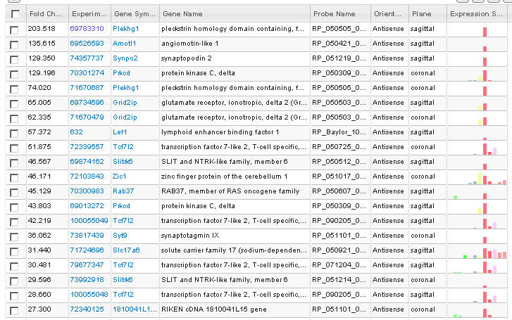
To perform a Correlation search, a user selects a seed SectionDataSet and a domain over which the similarity comparison is to be made. All voxels belonging to any of the domain structures form the domain voxel set. Pearson’s correlation coefficient is computed between the domain voxel set from the seed SectionDataSet and every other SectionDataSet in the Product. The return list is sorted by descending correlation coefficient.
Example: Correlation search for genes with similar expression to the sagittal Pdyn SectionDataSet
- Pipe: Set up the seed SectionDataSet by finding the sagittial SectionDataSet for gene Pdyn
- Connect the pipe to service::mouse_correlation to perform the correlation search
- Visualize the same search result in the Web application
See the connected service page for definitions of service::mouse_correlation parameters.
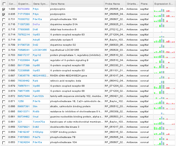
In order to perform these computations quickly over the entire data set, a subset of voxels are loaded in memory. The full expression grid is 67x41x58=159,326 voxels spanning both hemispheres and includes background voxels. To load all voxels for all image series into memory would require 14GB of RAM. To reduce memory requirements and increase the efficiency of calculations, voxels spanning over 80% of all experiments were identified. Only these ~26,000 voxels were then used in the ‘‘full’’ search service requiring 4 GB of RAM and partially spanning one hemisphere.
To take advantage the data on both hemispheres in coronal data, a second ‘‘coronal only’’ search service is also available as an option. The coronal service spans both hemispheres covering 58,387 voxels and searches over the ~4,000 coronal image series.
It should be noted that this on-the-fly search service is derived from a fully automated processing pipeline. False positive and false negative results can occur due to artifacts on the tissue section or slide and/or algorithmic inaccuracies. Users should confirm results with visual inspection of the ISH images.
Learn about Documentation Cell Types Database with comprehensive guides and examples from Allen Institute for Brain Science.
Available Files
Learn about Developing Mouse Reference Atlas with comprehensive guides and examples from Allen Institute for Brain Science.
Reference Datasets
To provide a neuroanatomical framework for gene expression data, the Allen Developing Mouse Brain Reference Atlas was created with the expertise of Professor Luis Puelles, M.D., Ph.D. (University of Murcia, Spain). Sagittal full-color, high resolution web-based digital reference atlases have been created for seven stages of mouse brain development accompanied by a systematic developmental taxonomy of mouse brain structures.
The Allen Developing Mouse Brain Reference Atlases were designed to:
- Allow users to directly compare gene expression patterns to an annotated developmental atlas;
- Provide templates for the creation of 3-D computer models of the developing mouse brain;
- Serve as a neuroanatomical foundation for informatics-based analysis tools.
In 2013, the reference atlas was updated to provide a deeper level of annotation. For more information on the reference atlas update and a description of the ontological levels, please refer to the Reference Atlas whitepaper located under the Documentation tab. Access to the previous reference datasets are available via links on the Reference Atlas landing page.
To access the reference atlas, you can click on one of the links from the landing page or you can select the key icon from the High Resolution Image Viewer to view the atlas in context with a gene expression experiment.
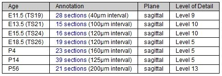
From the Reference Atlas landing page, you can also add reference data into your cart to enhance your exploration of gene expression data by clicking the checkboxes next to the desired reference dataset. Clicking “View Experiments” will allow you to view all selected datasets (including experimental data already present in the cart).
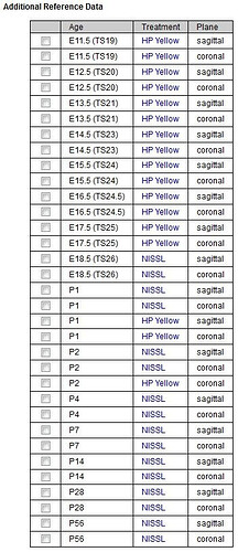
Translation Between the Adult and Developing Mouse Ontologies
Given there are two structure ontologies for the mouse brain in the Allen Brain Atlas resources, we have created a way to overlay the Structure Ontology from Adult Mouse Atlas and the Developing Mouse Brain Atlas.
While in the “Developing Mouse Atlas, P56”, select “P56 Adult Mouse” atlas from the second drop-down menu and select “Outlines” from the Tools icon drop-down. This will show both Structure Ontologies overlayed together.
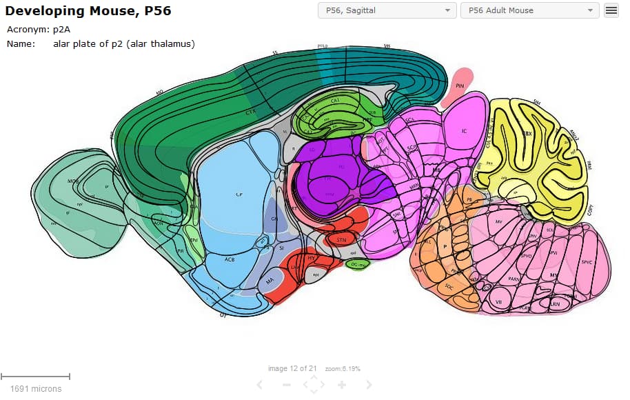
Reference Atlas Viewing with Gene Expression Data
Structure Ontology
The Structure Ontology for the Developing Mouse is listed hierarchically in the left-hand panel of the Interactive Atlas Viewer. By default the atlas is opened to level 3. Please see the Reference Atlas whitepaper available from the Documentation tab for more information on the Structure Ontology levels.
Each of the Developing Mouse atlases was drawn to a specific level and only those levels that were drawn will be available to navigate by clicking on the name. Those that are not available will be greyed out. Clicking on a structure name will take you to that drawn structure in the main image viewer.
Ontology Levels
Clicking on the ontology icon (see below) will open up the Developing Mouse Ontology defaulting at level 3.


The ontology levels in the Developing Mouse Atlas range from Level 00 (Neural Plate) up through higher differentiation levels to Level 13. Please see the Reference Atlas whitepaper available from the Documentation tab for a deeper explanation of the ontology levels. By clicking on the Ontology Levels (numbered squares above the ontology list) you will open the ontology to the level of detail indicated by the highlighted level.
Searching using the text box in the Ontology pane will allow you to browse through the ontology looking for specific regions. Using the “Sync” icon (see below), you can sync either image to its partner to view the gene expression in context with the reference atlas.
Given the difficulty of sectioning and programatically aligning these small specimen, you have the option of viewing a reference dataset with each gene expression specimen that will also outline a small structure of interest. To do this, choose the reference atlas from the Atlas dropdown menu (either Feulgen-HP or Nissl, depending upon the age) and select on the reference data set to outline your desired structure.
In the below image, gene expression is located in a region of the prethalamus.
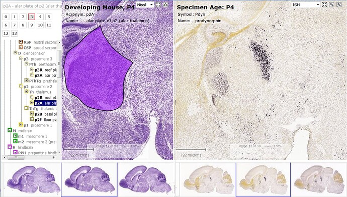
Reference Atlas Viewing Tools
Interactive Atlas Viewer (IAV)
Learn about Documentation Allen Developing Mouse Brain Atlas with comprehensive guides and examples from Allen Institute for Brain Science.
Available Files
Learn about In Situ Hybridization ISH Data with comprehensive guides and examples from Allen Institute for Brain Science.
Viewing Gene Expression Data
The Allen Mouse Brain Atlas offers the following ways for you to find gene expression data:
- Use Gene Search to locate genes’ data by name, symbol, NCBI accession number, or Entrez Gene ID.
- You can also use Gene Search with Boolean operators on specific field names using Boolean Syntax Query.
- Search for genes with enhanced expression by anatomic region using Differential Search.
- Search for manually curated enhanced gene expression data from 75 small structures using the Fine Structure Annotation.
- Differential Search across both the mouse and human gene expression datasets using the Human Differential Search.
- Search Related Studies for gene expression in our Sleep Study or our Mouse Strains Study.
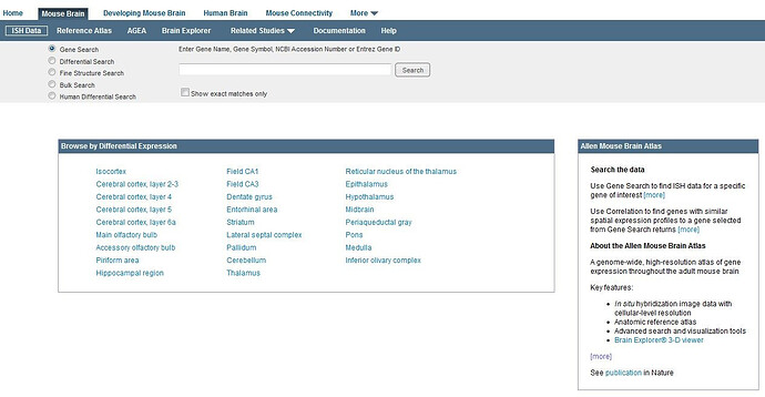
Gene Search
To search for a specific gene by name, symbol, NCBI accession number, or Entrez gene ID, type your query into the text box, making sure the “Gene Search” radio button is selected. As you type, genes that match your search string will be suggested to you. Select an item from the list and click the “Search” button. The results are displayed in a list that shows all genes with expression data that match your query.
Tips for searching:
- If you are unsure of spelling, begin typing the gene identifier and suggestions will be offered.
- Press the ‘Enter’ key instead of clicking the “Search” button.
- Include an asterisk (*) as a wildcard character before or after your search text to return genes that start with or end with that text. For example, enter pig* to return genes that start with pig or *pig to return genes that end with pig.
- If you do not include an asterisk (*) wildcard character, wildcards are implied to surround your search text. So if you search using the text pig, for example, you’ll get results that include pig anywhere within the gene name or symbol.
- Select the “Show exact matches only” check box to remove the implied wildcards. This is useful if you want to return only those genes that exactly match your search text.
- Place the search text within quotes to include spaces or special characters.
- Click the “Bulk Search” radio button to search for many genes at once. Doing so expands the text box, making it easier to copy and paste a list of genes from a text file or spreadsheet. Comma and semi-colon are not valid separators for genes; use tab or | instead. The bulk query does not implicitly include wildcard characters around your search text (you must specify them).
Boolean Syntax Query
The following special operators can be used to build queries:
- AND, OR and NOT must be upper case.
- The AND function is implicit, so spaces between words that are not separated by an operator will be treated like AND.
- OR has higher operator precedence than AND.
- Parentheses can be used to group criteria, but nested parentheses are not supported at this time.
Differential Search
The Differential Search option is ideal to search for gene expression data when the brain structure or area is known but little is known about genes that may be expressed in that area. To find genes with enhanced expression in one or more brain regions in contrast to one or more different regions, first select the “Differential Search” radio button. Enter the target structure(s) in the top search box labeled “Target Structure(s)” with a comma separating each structure. You can then enter “Grey” (for grey matter) or some smaller region as your contrast region in the “Contrast Structure(s)” search box, then click on the Search button.
The results are displayed as a list of genes with enhanced expression in the regions that match your query.
Differential search is an on-the-fly search service. Calculations over all ~25 000 experiments are computed as a fold change using expression energy data from one hemisphere. To restrict the search to coronal experiments (~4 000) which used data from both hemispheres, select the “Coronal data only” check box.
Since this search service is derived from a fully automated processing pipeline, false positive and false negative results can occur due to artifacts on the tissue section or slide and/or algorithmic inaccuracies. Users should confirm results with visual inspection of the ISH images. The “Expression threshold ” slider may be useful to reduce false positive results due to dark spot artifacts. This threshold restricts the list of returned results by excluding any experiment where the expression energy of the target structures is less than threshold.
Fine Structure Annotation
A differential search with manually curated results was generated for 75 small structures in the brain listing the top 50 genes with specific and enhanced gene expression. To use the Fine Structure search, select the “Fine Structure Annotation” radio button, then select a brain region from the drop down menu to return this list.
Human Differential Search
The “Human Differential Search” function enables side by side viewing and comparison of differential search across the mouse ISH and human microarray datasets. Select the “Human Differential Search” radio button. To find genes with higher expression in one structure compared to another structure, select a target brain structure in the top drop-down box and a contrast region in the bottom drop-down box and click on the Search button.
Search results
The return list is generated by first executing a differential search query in the mouse ISH dataset. Experiments for each gene are grouped together and ordered by maximum fold-change. For each gene in the mouse ISH return list, associated experiments in the human microarray dataset are identified; fold-change values are computed and displayed. Note that NCBI HomoloGene data is used to link genes across organisms. Click on the dataset column heading to toggle the primary dataset selection.
For each experiment, a gestalt visualization of the brain wide expression pattern is also provided. The type of visualization depends on the dataset:
For mouse brain data, expression is visualized as rotating 3D thumbnails. Each view is generated by maximum density projection where denser expression area appears more solid and obscures areas of lower density. Each cube is color-coded by average expression intensity ranging from blue (low intensity) through green to red (high intensity). Move slider bar in the header to rotate thumbnail.
For human brain data, microarray data is visualized as a heatmap where each column represents a tissue sample in ontological order. Heatmap color represents the z-score over a probe ranging from green (z-score of -3 and below) through black to red (z-score of +3 and above). Hover over any position in the heatmap to obtain the associated tissue sample structural annotation.

Correlative Search
In using gene expression databases, a “search by example” feature is also highly desirable as genes with similar expression patterns may be related in function. The Correlative Search utility will accomplish this function. This search by example facility is also available in the Allen Human Brain Atlas, Allen Developing Mouse Brain Atlas and the BrainSpan atlas of the developing human brain.
Once you have identified a gene of interest, to find other genes with spatial expression profiles similar to your gene of interest, first select your experiment by clicking on the gene name in the search results list. You will see that the experiment loads in the panel to the right hand side of the results list. Select the brain structure(s) in which you would like to see a similar expression pattern from the drop-down menu. You can search all the data or just the coronal data, by clicking the “Search Coronal Data Only” box, and click “Search”. This action will return experiments with a similar expression profile to brain region(s) in which you are interested.
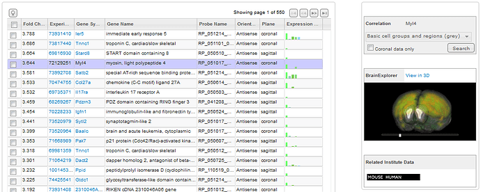
Viewing Search Results
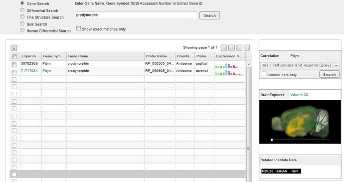
Searches will return a list of experiments based on the input search criteria. Each row includes the following information.
Select the experiments to view in greater detail by clicking on the checkboxes next to your experiments of interest. Experiments will be saved in your cache until you select the “Clear Selections” button at the bottom of the page. After selecting one or more experiments, click the “View Selections” button.
You can look for genes with a similar expression profile to your gene of interest by using the Correlative Search option: once a gene is selected, choose a structure from the drop-down menu and click “Search”. You can limit your results to only the data collected in the coronal plane by selecting the “Coronal data only” radio button.
Experiment Image Viewer
The experiment image viewer displays images for each selected experiment in a Zoom and Pan viewer. This view makes it easy to compare experiments with each other and with the Reference Atlas.
Multiple image series can be opened on the same page to enable side-by-side comparisons. Arrange the experiments by dragging a viewer by the title bar and dropping in a new location. Add a reference atlas by selecting one in the “Atlases” drop-down menu in the upper-right hand corner of the window.
If you are viewing more than one experiment, open the configuration options to change the number of columns displayed in the window. The configuration options are accessible by clicking on the button with a “gear” icon to the right of the “Atlases” menu.
The gene symbol is displayed in the title bar along with the Allen Institute image series ID. Additional details are displayed across the top of the viewing area, including the image index, tissue index, and tissue location.
Thumbnails for the entire image series are displayed across the bottom of the viewer in section order. Click a thumbnail to select it for viewing, or use the keyboard to navigate through the set. The current selection is outlined in black.
Experimental Detail
When the experiment is selected by clicking on the link, a summary of the experimental detail is returned. The data includes 1) an interactive 3-dimensional representation of gene expression, 2) a histogram of the expression energy in 12 different structures, 3) probe and gene metadata and 4) an interactive image viewer that displays the images in the experiment.
Hovering your mouse over the histogram will sync the image in the single image viewer with the section corresponding to that structure and expression.

Using the Zoom and Pan (ZAP) Image Viewer

The Zoom and Pan (ZAP) Image Viewer is a powerful tool to navigate and view the images in an experiment. The main part of the viewer is an interactive window where an image can be repositioned by dragging with a mouse. Use the scroll wheel or the keyboard to zoom in or out.
Select other images in the experiment by clicking on a thumbnail image below the main viewer.
Scale Bar
Drag the scale bar with your mouse to the desired location. Click on the text with your mouse to toggle between horizontal and vertical.
Using the ZAP Viewer Toolbar
Use the toolbar to take actions on the image that currently has focus. Toolbar controls include:
| Control | Function |
|---|---|
 | Move the slider bar to the left to intensify the contrast or color |
 | Select ISH, Nissl or Expression image type |
 | Display all thumbnail images in a single ‘contact sheet’ |
| Open the selected image in the image viewer tool |
| Synchronize all other Zap viewers on the page that support synchronization to the currently selected image |
| Open a new browser window to review metadata for the image series |
| Close the Zap viewer |
Keyboard Commands
Use the keyboard to navigate through the image series and synchronize the viewers on the page. Keyboard commands include:
You can also use the arrow keys to pan the current image.
Expression Energy
The expression mask image display highlights those cells that have the highest probability of gene expression using a heat map color scale (from low/blue to high/red).
The Expression Energy was calculated as follows: Within a given area A (voxel or structure), expression energy = (sum of intensity of expressing pixels in A) / (sum of all pixels in A)
Using the High Resolution Image Viewer
The image viewer enables you to view a high resolution image in its own re-sizable window. It is possible to open multiple images by opening multiple windows.

Ways to interact with an image include:
- Use the on screen navigation buttons to zoom, pan and move forward or backward through the image series. You can also use the Keyboard Commands used in the ZAP Image viewer.
- Drag the scale bar with your mouse to the desired location. Click the text with your mouse to toggle between horizontal and vertical.
- Use the Configuration Menu to download images and adjust image parameters.
- Use the Interactive Atlas Viewer to view the reference atlas along side the ISH images
Learn about Allen Developing Mouse Brain Atlas Supplementary Data with comprehensive guides and examples from Allen Institute for Brain Science.
Archived Documents
Archived March, 2010
The reference atlas and ontology were updated in June, 2013. The following archived documents from the versions released in March, 2010.
Note: The E11.5, E13.5, and E15.5 reference atlas files may be too large to open in your browser. For the best results, save the files locally and open them with a PDF viewer.
Archived April, 2009
The following archived documents were the first versions released in April, 2009.
Learn about Anatomic Gene Expression Atlas AGEA with comprehensive guides and examples from Allen Institute for Brain Science.
What Is AGEA?
The Allen Institute has built a data-driven three-dimensional atlas of the adult C57Bl/6J mouse brain based on the ISH gene expression images of the Allen Mouse Brain Atlas. Only the coronal gene expression data were used to construct this application. The AGEA feature (which stands for Anatomic Gene Expression Atlas) characterizes the multi-scale spatial relationship in the mouse brain as derived from coronal gene expression data without a prior knowledge of classical anatomy. Using the AGEA feature of the Allen Mouse Brain Atlas, you can:
- View and navigate 3-D spatial relationship maps (Correlation mode) and search for genes within the coronal dataset with local regionality (Find Genes) and,
- Explore a transcriptome based spatial organization of the brain (Clusters mode).
To launch this feature, click on the AGEA tab from the Allen Mouse Brain Atlas and you will see the following image.
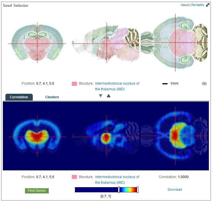
The upper panel of images are orthogonal views of a 3-D Nissl reference atlas volume. The reference space was divided into 200 µm volumes, or voxels. The cross hairs in the top panel of images select for a seed voxel from which to compare to gene expression profiles to all other voxels in the brain. For more detailed information on how AGEA was constructed please see the AGEA user guide or Ng L, et al.(2009) An anatomic gene expression atlas of the adult mouse brain. Nature Neuroscience 12(3): 356-362.
The AGEA Viewer
This section describes the controls for the Correlation and Cluster modes of AGEA.

A. Seed Selector panel: Use this area to select the seed voxel as marked by the red crosshairs. Either click or click and drag to navigate to a different correlation map.
B. Map panel: This area displays the three orthogonal views of the currently selected correlation map in coronal, sagittal and horizontal planes. The red crosshair marks the currently selected voxel. Either click or click and drag to move to a new 3-D location. Note that this volume can be navigated in 3-D for any selected voxel location from A.
- About/Permalink/Zoom: Clicking on “About” will bring up more information on AGEA, clicking on “Permalink” creates an URL in the address bar that effectively saves information about your current viewing state. This URL can be saved for later access to directly take you back to the current view and color scale settings. Clicking the arrows will toggle between zooming the images to fit in the window and a higher resolution, more zoomed mode. At a fixed zoom level, you may need to use the browser scroll bars to view all the images.
- Mode Selector: Click on Correlation or Clusters to switch the viewer to different modes.
- Position: The position of the seed selector crosshairs in millimeters in PIR (+x = posterior, +y = inferior, +z = right) orientation, where the origin is the anterior, superior, left corner of the volume.
- Lock/Sync: The icon on the left locks the planes shown in the selected expression map B to the same position as the seed map A. Click to toggle the locking behavior. Conversely, click on the right icon to move the seed voxel to the current selected map voxel.
- Allen Reference Atlas Label (Panel A): The structure or structural grouping from the Allen Reference Atlas to which the seed voxel (indicated by red crosshairs) belongs. Click on the name to open a window with an interactive reference atlas viewer.
- Allen Reference Atlas Blend: This icon toggles blending Allen Reference Atlas structural delineations on the Seed Selector images for direct anatomic comparison.
- Position: The position of the seed selector crosshairs in millimeters in PIR (+x = posterior, +y = inferior, +z = right) orientation, where the origin is the anterior, superior, left corner of the volume.
- Allen Reference Atlas Label (Panel B): The structure or structural grouping to which the selected voxel (indicated by red crosshairs) belongs. Click on the name to open a window with an interactive reference atlas viewer.
- Correlation: Value of the correlation at the currently selected voxel with respect to the seed voxel selected in panel A. This shows numerically how well the target voxel is correlated with the seed.
- Gene Finder Button: (in Correlation mode only) Click this icon to find genes with enhanced expression in the voxel targeted by the crosshairs in panel A.
- Color scale control: Use to adjust the false color mapping of the correlation map to threshold the images for regions of higher significance. All voxels with correlation within the select range are rescaled to span the color scale.
- Download: Click to download the currently selected correlation map as raw flat file with numbers saved as floats.
Using Correlation Mode
In Correlation mode, the lower panel shows orthogonal views of the selected spatial relationship map. The correlation values in the bottom figures can be interpreted as a measure of average co-expression between two voxels. The higher the correlation value between voxels, the more common it is for genes from the seed voxel to be co-expressed. Higher correlation between two voxels indicates more spatial correlation of expression and thus potentially higher possibility that the spatial regions spanned by the voxels are anatomically related. This may indicate that the voxels compared share common cell types or represent a coherent functional map. The correlation map can also be used to locate coexpressing areas in other brain regions. In the above figure, the map indicates that there is higher co-expression in thalamic structures than in other regions of the brain.
When a seed voxel is selected using the crosshairs in the images from the top panel, you can find correlations between the seed voxel and other voxels in the brain by selecting a distinct voxel in the lower panel using the crosshairs in the images from the lower panel. The correlation between the regions will be displayed below the lower panel (9).
The gene finder search facility is among the most powerful aspects of AGEA’s functionality. It enables users to search an anatomic region of interest for genes within the Allen Mouse Brain Atlas coronal database that exhibit localized enrichment. Clicking the “Find Genes” button returns a list of genes selected by the crosshairs in the upper panel (A). Voxels in the yellow to red range (top third of the range) are considered the local region of interest (target domain) while all voxels above threshold cutoff (all non-dark blue voxels) forms the contrast domain region. These domains are used in the differential search to find the genes that exhibit localized enrichment.
Gene Finder Search Results
Clicking the “Find Genes” button will return a list of experiments based on the input search criteria on a separate page. The AGEA correlation map as well as the seed location in PIR orientation (in µm) is illustrated at the top of the page.
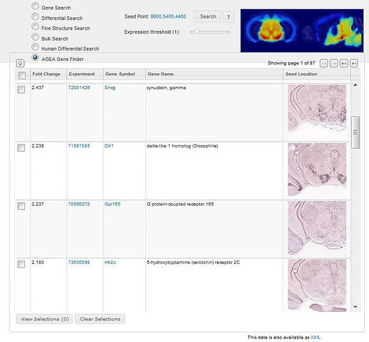
Each row of the search results includes the following information.
| Column | Description |
|---|---|
 | Add the experiment to your selections by clicking the checkbox |
| Fold Change | A numeric value representing the fold change between expression of the target domain and the contrast domain |
| Experiment ID | Click the experiment number to view experimental detail page |
| Gene Symbol | Click Gene Symbol to return gene metadata |
| Gene Name | Full gene name (click to see 3-D thumbnail and perform a NeuroBlast search) |
| Seed Location | Image from the seed location |
You will have to visually inspect the dataset to ensure the signal that AGEA detected was real and not an artifact of the image collection.
Clusters Mode
Selecting Clusters mode switches the lower panels to view a data-driven hierarchical binary tree spatial organization of the brain computed from the AGEA correlation maps. To construct the decomposition, all 61,053 voxels were assigned to the root node of the tree. As we descend the tree, a node is bifurcated into two nodes to achieve maximal dissimilarity between two groups of voxels based on correlation values. The final bi-tree consists of 122,105 nodes with a maximum depth of 54 levels and 61,053 leaf nodes (one for each voxel in the brain). Effective visualization of this large data structure is via an easy-to-use Tree Depth slider mechanism to navigate the bi-tree, providing 3-D context and visualizing the multi-scale partitioning.
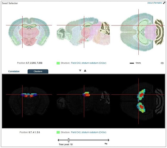
In the above example, when the field CA3 is selected from the top panel you can see the relationship of this region to the rest of the hippocampal formation at a tree depth of 10.
The voxels of a node are visualized with a systematic color coding scheme. All voxels of a node are assigned a color based on the ‘jet’ color scheme where the leaf node with low-order voxels are assigned shades of blue. The colors then run through green, yellow, orange, and finally, higher-order voxels are assigned shades of red.
Learn about How To Brain Explorer with comprehensive guides and examples from Allen Institute for Brain Science.
Brain Explorer® 3-D Viewer is an application for viewing brain anatomy and gene expression data in three dimensions in the framework of the Allen Reference Atlas.
Using Brain Explorer, you can:
• View a fully interactive version of the Allen Reference Atlas in 3-D.
• View gene expression data in 3-D at 200 µm 3 resolution.
• View expression data from multiple image series superimposed on each other in 3-D.
• Navigate the high-resolution 2-D ISH images using the 3-D model.
• Link to associated gene metadata on the Allen Mouse Brain Atlas web application.
Installation
Windows
Systems requirement: minimum configuration
• Operating System: Microsoft Windows 7
• CPU: Intel Core Duo or AMD 1.8GHz
• System Memory: 1GB
• Graphics Card: Hardware 3D OpenGL accelerated AGP or PCI Express with 64MB RAM
• Screen: 1024x768, 32-bit true color
• Hard Disk: 200MB free space
Note: Brain Explorer is known to work with the following video chipsets: nVidia GeForce 9400/9600, nVidia Quadro FX 1800/3800/5600, AMD Radeon 9600, AMD Radeon HD 3200/4550, Intel Q35/Q45 Express.
For the best performance, please check with your video card vendor for the latest available drivers before using Brain Explorer. The Windows version of the Brain Explorer viewer is available here. Double-click the downloaded BrainExplorer2.msi file and follow the prompts.
Mac
Systems requirement: minimum configuration
• Operating System: OS X 10.6.8
• CPU: Intel 1.8GHz
• System Memory: 1GB
• Graphics Card: 3D-capable with 64MB RAM
• Screen: 1024x768, 32-bit millions of colors
• Hard Disk: 200MB free space
Note: Please install the latest system updates from Apple to ensure you have the latest video card drivers.
The Mac version of the Brain Explorer viewer is available here. Double-click the downloaded zip file to unpack Brain Explorer.
Installing Atlases
A one-time download containing anatomy files is needed following installation of the Brain Explorer application. The first time you open the Brain Explorer software, you will be asked to choose to download files for the Allen Developing Mouse and Allen Human Brain atlases. Click on the atlases you would like to use and then click the Install button.
To download missing atlases on the PC, go to the Help menu and select Download Atlases. On the Mac, the command is in the Brain Explorer 2 menu.
Getting Updates
The Brain Explorer application will inform you when updates to the Brain Explorer application itself or its atlases are available. New data may not be available for viewing until you install the required updates.
Viewing Gene Expression
To load gene expression data into the Brain Explorer viewer: go the Allen Mouse Brain Atlas and perform a gene search. You can type in a gene in the search box or click on a structure name to retrieve differential enriched genes. Your search brings back a list of experiments. Click on a row to select an experiment of interest. A 3D thumbnail of the expression pattern of that experiment will appear to the right. Click on the blue “3D” file link to launch the Brain Explorer application.
When the Brain Explorer 3-D Viewer opens, you will be taken to a screen that displays the Image Viewer, the Structure Ontology Viewer, and the Gene List.
Image Viewer
The Image Viewer will automatically show the 3-D expression representation of your selected experiment. Each sphere represents expression re-sampled to a 200 micron grid resolution. Larger sphere corresponds to a greater density of expression.
You can select a sphere by clicking on it. Spheres can be deselected by clicking on blank space. The original ISH image of the selected sphere will be displayed blended with the expression heat mask in the lower left hand portion of the screen. The blending can be adjusted by selecting Image Controls from the View menu and moving the Image Blending slider. Double-clicking on the zoomed ISH image will open the corresponding ISH image in a high resolution image viewer.
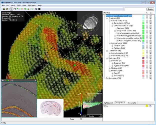
The information at the upper left corner of the main Brain Explorer window summarizes the expression detected in the selected grid location. These numbers include the average expression density and intensity (over pixels). The Informatics Data Processing White Paper describes how the measurements were obtained.
To change the gene expression representation, click on the “Data” menu and select an option under “Raw” colors.
A compass in the right-hand corner of the Image Viewer can be used to rotate the brain by clicking and dragging your cursor. You can zoom using either the wheel on your mouse or using the Zoom scrollbar in the lower right hand corner of the Image Viewer.
Expression Thresholds
A way to control expression visibility is by setting thresholds on expression values. This method can restrict visible spheres to different combinations such as low intensity and low density or high intensity and low density.
The graph in the lower right hand corner shows a dot for each data point (sphere) in a gene expression file, and the color of the dot corresponds to the anatomic annotation in the same way the atlas colors display mode works. Each data point is plotted according to its density on the x axis and its intensity on the y axis.
The color scale on the left-hand side of the graph corresponds to the expression level heat map used to color the spheres. The numbers along each axis show the values at the yellow triangles.
The thresholds can be changed by resizing the white box. Any edge or corner of the box can be clicked and dragged to re-size it. You can also click and drag in the center of the box to move the box.
Structure Ontology Viewer
The Structure Ontology Viewer shows the entire collapsible ontology for the mouse brain as defined by the Allen Reference Atlas. Two columns to the right of the ontology determine the type of data displayed in the Image Viewer. “A” represents atlas structure and when checked, will show a visual representation of that structure in the Image Viewer. “D” represents gene expression and when checked, will show gene expression in that structural domain.
The default organization for the Structure Ontology is the Hierarchical View, but if you are unfamiliar with the ontology, you can click on the Alphabetical View to see the structure list in alphabetical order.
The Bookmarks tab is a space where you can create and save favorite views of the brain. Several default views are already saved that will rotate the brain back into common viewing frames.
Gene List
This section displays the gene probes you have selected and downloaded in this session. Right clicking on the gene probe name will bring up a menu where you can, 1) view the gene detail page (Get Info), 2) be taken to a zoomed-in image from this experiment (View Images), 3) copy meta information to the clipboard, such as symbol, name, Entrez ID, image-series ID (Copy Info), 4) activate a Correlation search, finding experiments with similar expression profiles (Find Similar) or 5) close the experiment and remove it from the list and the 3-D view (Close).
Gene Search
To search for genes within the Brain Explorer application: go to the Search box located above the ontology panel and type in the gene symbol or part of a gene name.
The list of results shows gene name, gene symbol along with a 3-D summary thumbnail of the expression for each experiment matching the search. The expression thumbnail represents a maximum expression projection rendering: the denser the expression in a region, the more “solid” the appearance. Reference atlas colors are additionally layered on top.
To load an experiment for viewing click on the “Download” button under the gene name.
Advanced Features
Atlas Menu:
You can show opaque three dimensional structures of the brain by “showing” or “hiding” structures from this menu. The “Transparent” function allows you to see transparent views of the structures to view the anatomical relationships between them.
Selecting the sagittal, coronal or horizontal sections (or clicking on one of the section image buttons in the toolbar) will superimpose a single plane of the MRI images from each brain on your image space. These planes can be moved once the selection tool mode button in the toolbar is selected. Selecting “Show Annotation on Sections” from this menu will color the MRI images, if any are available, according to the brain structure ontology.
Select “Show Full Resolution Image” to link to the high resolution annotation reference atlas images.
To find genes enriched in particular structure: select a structure in the ontology tree then select “Find Genes” in the Atlas menu. This uses the same “Differential Search” functionality as the web application.
Data Menu:
When you have a gene selected, the Data menu allows to you to show all expression, hide all expression (for instance to then select a single structure) or toggle expression (for instance, unselect your region of interest then toggle to see expression in only that region).
You can also show or remove threshold controls and choose the visual representation of your data from this menu. There are several options under “Raw” colors:
• User defined: Each experiment is rendered in user specified color. This mode is useful to distinguish between individual experiments when multiple experiments are being displayed.
• Atlas: In this mode the sphere is colored by the corresponding reference atlas structure color. This mode is useful for quickly seeing the annotated regions where a gene is expressing.
• Expression Level: This mode displays average expression intensity and is useful for identifying areas of very high expression.
• Jet: Applies the common “jet” colormap to the data.
To be taken to the experiment detail page, select “Get Info”. To explore the images in this experiment, choose “View Images”. These functions are also available by right-clicking on the gene name in the Gene List.
Choose “Find Similar” to find similar genes to the selected experiment. This uses the same Correlation search functionality as in the web application.
Clipping Planes:
When this function is selected, either by toggling the cutting tools button in the toolbar or selecting “Clipping Planes” from the View drop down menu, you can make coronal, sagittal or horizontal cuts in your view of the brain and related data. To cut in a particular plane, make sure the cursor is in selection tool mode, and then click and drag on the plane you are interested in clipping.
Troubleshooting
Windows
Graphics
If you are using a desktop computer, you should obtain drivers from the video card manufacturer. First, identify the video card. Go the Start menu and open the Control Panel. Open the Display control panel and go to the Settings tab. Click the Advanced button and go to the Adapter tab. Your video card vendor and model name will be displayed at the top of the window under Adapter Type. Please go to the manufacturer’s web site, locate the driver download, and follow the instructions on the website or included with the downloaded file.
If you are using a laptop computer, you will need to go to your laptop manufacturer’s web site to locate the latest video drivers.
You can also activate an alternate drawing mode in Brain Explorer. Go to the View menu and select Options. Check the Draw faster but at lower quality button and uncheck the Synchronize drawing with the monitor’s vertical refresh button. Set the Multisample setting to Off.
If you are using multiple video cards from different vendors, the 3-D display may not work correctly on all attached monitors.
Uninstalling
Use the Add/Remove Programs control panel or the uninstall link in the Brain Explorer folder in the Start menu. Additional data that are not automatically uninstalled are located at the following locations:
Windows XP
Atlas data: C:\Documents and Settings\userid\Local Settings\Application Data\Allen Institute\Brain Explorer 2
User settings: C:\Documents and Settings\userid\Application Data\Allen Institute\Brain Explorer 2
Windows Vista and Windows 7
Atlas data: C:\Users\userid\AppData\Local\Allen Institute\Brain Explorer 2
User settings: C:\Users\userid\AppData\Roaming\Allen Institute\Brain Explorer 2
Proxy Settings
If you use a proxy server, the Brain Explorer application will use the proxy settings from the Internet Options control panel in the Windows Start menu. Please refer to the Windows documentation for help on proxy settings.
Mac
Uninstalling
Drag the Brain Explorer 2 icon to the trash. The Brain Explorer application generates the following files, which can also be dragged to the trash.
- ~/Library/Application Support/Brain Explorer 2
- ~/Library/Preferences/org.alleninstitute.BrainExplorer2.plist
Performance
If the Brain Explorer application is not running smoothly, first try to free up as much memory as possible by quitting all other open applications. You can also activate an alternate drawing mode. Go to the Brain Explorer 2 menu and select Preferences. Check the Draw faster but at lower quality button and uncheck the Synchronize drawing with the monitor’s vertical refresh button. Set Multisampling to Off.
Learn about Documentation Allen Mouse Brain Atlas with comprehensive guides and examples from Allen Institute for Brain Science.
Available Files
Learn about Related Studies To Mouse Brain Atlas with comprehensive guides and examples from Allen Institute for Brain Science.
Sleep Study
The Allen Institute partnered with SRI International to examine the effects of sleep deprivation and sleep state in mice. Approximately 200 genes were assayed in this study. The experimental conditions include:
To view the data in this study, select “Sleep” from the “Related Studies” drop-down menu in the banner.
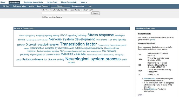
To search for a gene, either select one of gene categories from the tag cloud, or type the gene name into the search box. As you begin to type, a list of suggestions will be displayed and you can select from the list of available genes. A list of relevant experiments will be displayed based on your search criteria.
Search Results
Results of your search will be displayed as a list of experiments based on the input search criteria. Each row includes the following information.
| Column | Description |
|---|---|

| Add the experiment to your selections by clicking the checkbox |
| Experiment | Click the experiment number to view experimental detail page |
| Gene Symbol | Click Gene Symbol to return experimental detail pages for all experiments using that gene |
| Gene Name | Full gene name |
| Probe Name | Unique identifier for the probe used in this experiment |
| Condition | An abbreviation of the experimental condition (hover over the condition to see full description) |
| Expression Summary | Thumbnail view of a histogram showing the expression energy across 12 major brain structures |
Once you have selected experiments to view (by clicking the checkbox), click “View Selections” to explore the experimental images further.
Mouse Strains Study
The Mouse Strains Study (previously known as the Mouse Diversity Study) provides gene expression data from a select number of genes across seven different mouse strains and in adult female C57BL/6J mice, expanding upon the original Allen Mouse Brain Atlas.
To view data in this study, select “Mouse Strains” from the “Related Studies” drop-down menu in the banner.

To search this data, either click on the gene symbol in the tag cloud to bring up all the data related to that gene, or type in your gene (from the tag cloud) and filter your search by strain, gender and/or plane of sectioning and click “Search”.
Search Results
Results of your search will be displayed as a list of experiments based on the input search criteria. Each row includes the following information.
| Column | Description |
|---|---|
| Column | Description |
|
| Add the experiment to your selections by clicking the checkbox |
| Experiment | Click the experiment number to view experimental detail page |
| Gene Symbol | Click Gene Symbol to return experimental detail pages for all experiments using that gene |
| Gene Name | Full gene name |
| Sex | Gender of the Mouse line, either M or F |
| Probe Name | Unique identifier for the probe used in this experiment |
| Strain | Strain of the mouse used in the experiment |
| Plane | Plane of sectioning, either coronal or sagittal |
| Expression Summary | Thumbnail view of a histogram showing the expression energy across 12 major brain structures |
Selecting the “Show exact matches only” box will limit your search to exactly what you type in the Search box. If you select the “Update results when criteria change” box, clicking on the advanced search parameters will automatically update the experiments returned in your search results. Once you have selected experiments to view (by clicking the checkbox), click “View Selections” to explore the experimental images further.
Learn about Projection Dataset with comprehensive guides and examples from Allen Institute for Brain Science.
Searching
The Adult Mouse Connectivity Atlas comprises a searchable image database of axonal projections labeled by viral (rAAV) tracers and visualized using serial two-photon tomography.
Search this dataset using:
1. Source Search which allows searching by injection site (Filter source Structure(s)) and filtering by mouse line, tracer type and the presence of Intrinsic Signal Images

2. Target Search a “virtual retrograde” search that finds experiments based both on injection site and projection through a structure of interest
3. Spatial Search a spatial search allows the user to choose either a target signal or injection site based on selecting a voxel through which signal passes

There are example searches in the Browse Data subject box on the landing page to demonstrate the various ways in which relevant data can be found. You can also browse experiments from the 3-D search result visualization. Hovering your mouse over the dots (colored according to the Reference Atlas) NEED LINK HERE will indicate the primary injection structure of that particular experiment.
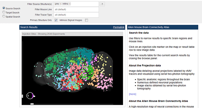
Please see the Informatics Data Processing whitepaper available in the Documentation tab for more information on the informatics processing performed in this study.
Source Search
The default view is all experiments throughout the brain (indicated by “grey” and “retina”). To filter your search by injection site, select a structure(s) from the structure ontology that opens when you click in the “Filter Source Structure(s)” text box.
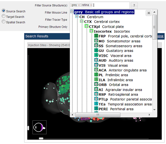
From the Source Search, you also have the option to filter by mouse line or by tracer type. To filter by mouse line, click in the “Filter Mouse Line” text box and select from Wild Type, Cre line or Ai75(RCL-nt) options, or start typing in the text box to search tags from the various Cre-dependent mouse lines. The Ai75 (RCL-nt) option is a reporter strain that we used to target neurons within certain regions. When filtering using the “Filter Tracer Type” text box, you will have the option to choose between EGFP (axonal EGFP) experiments, SypEGFP (synaptophysin-tagged, synaptic EGFP) labeled experiments, or Target EFGP experiments. For more information on this targeting strategy, please see the Overview whitepaper in Documentation.
Although every effort was made to limit the injection site of the viral tracer to a single brain structure, it was often the case that cells in neighboring structures were also infected. We refer to these as “secondary injection structures” and include them in the results list as they may also contain interesting scientific information. To view these experiments as well, uncheck the “Primary Structure Only” box.
As we precisely target the higher visual areas in this data set, experiments utilized Intrinsic Signal Imaging for both guiding injections into the visual cortex, as well as to inform the interpretation of projection pathways. To view experiments that include these data, check the Intrinsic Signal Images box.
As you select filtering parameters, notice that the number of experiments in the 3-D search result visualization decreases to show only the number of experiments that fit your search criteria.
Below the 3-D search result visualization, a list will automatically load with all the experiments that fit your filtering criteria.
This list includes:
Clicking on the column headings will sort the list of experiments by that column, clicking twice on a single column will reverse the sort order. Once you have found a relevant group of experiments, you can save or bookmark these search results using the “Permalink” function.

Several experiments can be selected to view side-by-side and/or in the context of our reference data by checking the boxes next to the experiments. Once you have selected the experiments you want to view, click the “View Selections” button. Those experiments will be available in your cart to view in the Experiment Image Viewer until you clear your cache or click the “Clear Selections” button.
Once you have narrowed your search and want to delve deeper into an individual experiment, open the Experiment Summary View by clicking on a circle in the 3-D search result visualization or an experiment in the list.
Target Search
This search has all the same functional capabilities as Source Search with the added ability to filter your search by limiting the results to experiments where the projection signal passes through a given structure(s).
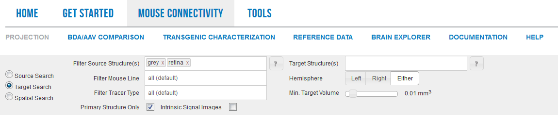
By default, when you click the “Target Search” radio button, the “Target Structure(s)” search box will open. After selecting one or more structures, selecting a hemisphere, or changing the minimum target volume (defaulted to 0.01 cubic mm), the 3-D search result visualization will automatically update with experiments that fit your filtering criteria. The list of experiments under the 3-D search result visualization includes the following information:
Experiments are sorted by the target volume, but can be resorted by clicking on a column header. Once you have found a relevant group of experiments, you can save or bookmark these search results using the “Permalink” function.
Several experiments can be selected to view side-by-side and/or in the context of our reference data by checking the boxes next to the experiments. Once you have selected the experiments you want to view, click the “View Selections” button. Those experiments will be available in your cart to view in the Experiment Image Viewe until you clear your cache or click the “Clear Selections” button.
Once you have narrowed your search and want to delve deeper into an individual experiment, open the Experiment Summary View by clicking on a circle in the 3-D search result visualization or an experiment in the list.
Notice that experiments in the retina can be highlighted by hovering over the eye in the lower left-hand corner of the 3-D visualization or can be selected by clicking on one of the spheres indicating the entry point into the brain.
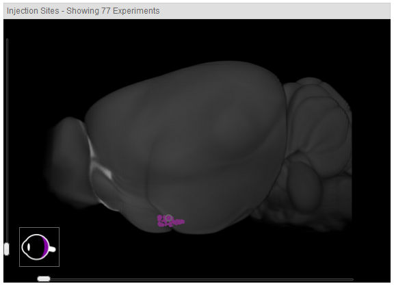
Spatial Search
Clicking the “Spatial Search” radio button allows you to do a voxel-based “virtual retrograde” search, or search for injection sites in close proximity to a selected voxel. The default view is pointed to a voxel in the ventral posterolateral nucleus of the thalamus, as indicated by the cross hairs in the multiplanar viewer. The 3-D search result visualization depicts all the injection sites with projection signal through the chosen structure. The approximate injection site is depicted with a sphere and the approximate pathway is traced with a line the same color as the injection site.
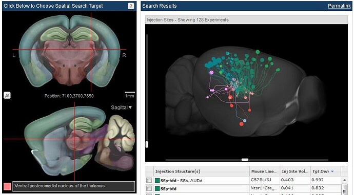
Selecting the “Find Injection Sites” filter will bring up a threshold bar that will allow you to search for injection sites within a specified distance from your cross-hair location.
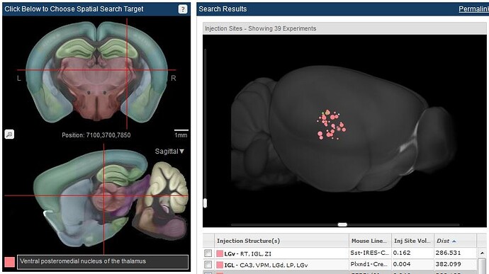
Click and drag the cross hairs in the multiplanar viewer to select a voxel in a particular structure. Once you have chosen a structure, you can further filter your search by selecting a mouse line and/or filtering by primary injection structure. The resulting list of experiments will include:
Using the Multiplanar Viewer to Search
The voxel-based Spatial Search is carried out by using the multiplanar viewer. This viewer illustrates the Allen Mouse Common Coordinate Framework (CCF) and incorporates structures drawn in 3 dimensions: see the Mouse CCF whitepaper in Documentation. Access to the horizontal view is via the drop-down menu in the sagittal view.
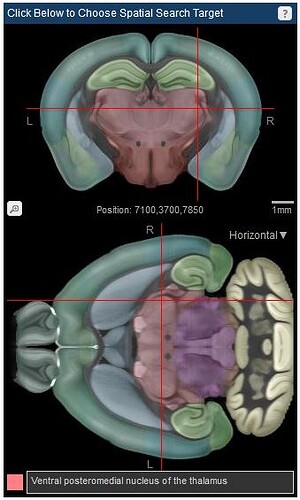
Experiment Summary View
Hovering your mouse over an experiment will highlight that injection site in the 3-D search result visualization. Rotating the image in either the horizontal or vertical planes gives better access to view the selected experiments. To take a closer look at a particular experiment, click on that experiment, either in the list or on the 3-D search result visualization. Once an experiment has been chosen in this manner, a new panel of images and options will load on the right labeled by the Experiment ID number and the injection site structure. This view includes a section images viewer, a projection density image viewer, a transgenic characterization box, an injection summary for the rAAV virus injection and the targeting CAV injection summary (when appropriate) and a correlative search box. Characterization of the transgenic lines used in this study has been carried out, and can be inspected from the link in the Transgenic Characterization box. If viewing an experiment from the Retinal Projectome, a whole mount view of the retina is available from a link in the Transgenic Line box. Experiments that show a similar signal pattern to the current experiment can be searched for using the Correlative Search.
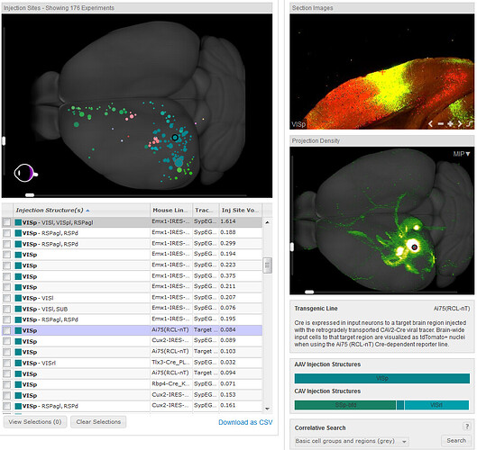
Advanced search features are available from the icons in the toolbar of the experiment panel and include:

Open the experiment in a Cortical Map Viewer also where Intrinsic Signal Images (when available) will be displayed

Shortcut key to conduct a Spatial Search from the point indicated by the cross hairs

Open the experiment in the 3-D Brain Explorer software

Open the experiment in a High Resolution Image Viewer

Open quantification of the signal in the Experimental Detail page
Section Images Viewer

The section images viewer shows the 2-D fluorescence images in both the green (signal) channel and the red (autofluorescence) channel. Navigation (panning and zooming) through these images is achieved by using the on-screen navigation tools or using the Keyboard Commands. This project utilizes extensive informatics processing and the informatics signal calculated by subtracting the background signal (segmentation images) can be viewed by clicking the icon (see below).

Projection Density Image Viewer
This view shows an interactive 3-D thumbnail view of the experiment in what is referred to as the Maximum Intensity Projection (MIP) view. By default, a cross hair and sphere indicates the center of the injection site. Clicking on any other position in the MIP view will move the cross hair to the site selected both in the MIP view as well as in the 2-D view in the section image view. As selecting a point in a 3-D image can become problematic, you also have an option to view the intensity projection in 2-D from the drop-down menu that opens when you click on “MIP”. These views show the signal intensity against the two dimensional view of the Allen Mouse Common Coordinate Framework (CCF). For more information on the CCF, please see the whitepaper in the Documentation tab.
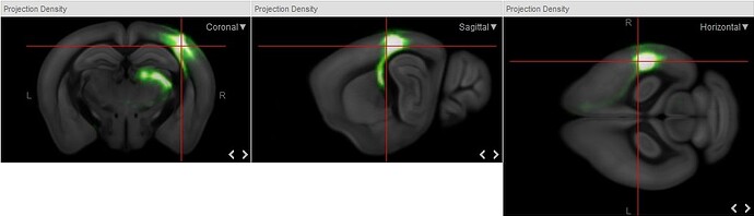
The left (L) and right (R) sides of the brain are labeled in these views and navigation to the next section is achieved by clicking the < and > on-screen navigation buttons.
An example of the segmentation view is illustrated in the image to the right. For more information on the informatics processing in this project, please see the Informatics Data Processing whitepaper available from the Documentation tab.
Correlative Search

Once you have found a relevant experiment, another useful search is for any other experiments that may show similar projection patterns. The correlative search allows you to look for similar patterns with an experiment of interest either by comparing brain wide (default), or by selecting fiber tracts or one of the other 12 major curated brain divisions available from the drop-down menu.
Cortical Map Viewer
In order to enable the integration of information from different cortical depths, we constructed a curved cortical coordinate system. This coordinate system allows us to project structural features in the cortex, which are often oriented orthogonally to the surface, in a two dimensional plane that preserves structural integrity. When viewing projections in the Cortical Map, you are viewing the cortex along a “streamline” (see figure below and CCF whitepaper in Documentation.
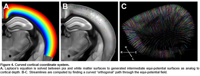
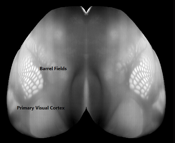
When viewing this curved cortical coordinate system in two dimensions, structures such as the barrel fields in the somatosensory cortex and the primary visual cortex become visually distinct. While the curved cortical map nicely delineates the primary visual cortex, the associated visual areas are not so easily mapped. To further delineate these areas, Intrinsic Signal Imaging was performed during a visual stimulus to create sign maps for each individual brain.
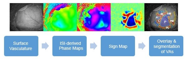
For more information on how the sign maps were generated, please see the Overview whitepaper in Documentation. The March 2016 data release was the first to include experiments that used sign maps to both target infection to specific visual areas as well as interpret projection from other brain regions to the visual areas.
Viewing Projection Experiments
Experiments without Intrinsic Signal Imaging (ISI)
When viewing an experiment of interest, you can visualize that experiment in the cortical map by clicking on the cortical map icon.
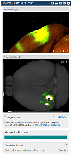
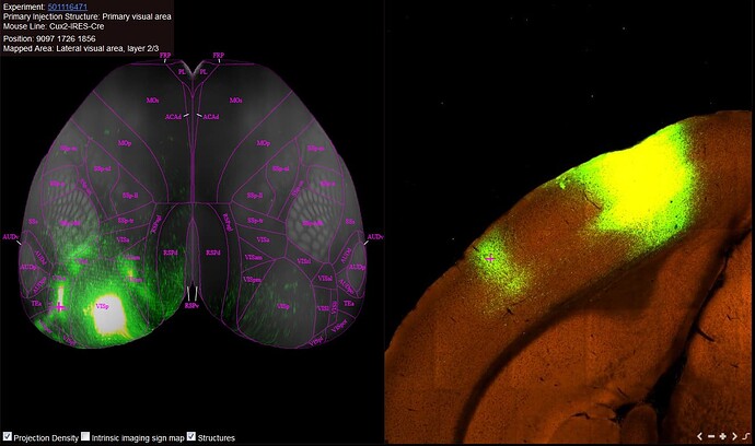
Note: only the projection signal in the cortex is visible in the Cortical Map viewer.
The cross-hairs on the Cortical Map indicate the location of the 2-D image from the experiment to the right. Navigation to other locations in the experiment is from either the on-screen navigation icons, or by double-clicking on the Cortical Map itself. Once a location has been chosen, the experimental ID, primary injection site, mouse line, position (in microns) and the location mapped to the reference atlas will show up in the left-hand corner of the screen. Clicking on the experimental ID link will take you to the Experimental Detail Page. Only the Projection Density and Structures checkboxes will be available for experiments without ISI.
Experiments including Intrinsic Signal Imaging (ISI)
To see experiments that include ISI, make sure to check the “Intrinsic Signal Images” box in your initial search.
Once an experiment with ISI has been selected, a radio button will appear which allows overlay of the projection and ISI views.

The cross-hairs on the Cortical Map indicate the location of the 2-D image from the experiment to the right (not shown). Navigation to other locations in the experiment is from either the on-screen navigation icons, or by double-clicking on the Cortical Map itself. Once a location has been chosen, the experimental ID, primary injection site, mouse line, position (in microns) and the location mapped to the reference atlas will show up in the left-hand corner of the screen. Clicking on the experimental ID link will take you to the Experimental Detail Page.
Experimental Detail Page
The experimental detail page illustrates the projection experiment in an informatically quantified fashion. This page contains the Injection Summary(ies), a Projection Density Image Viewer, a Section Images Viewer, and a histogram quantifying the signal in each region, displayed either by Projection Volume or Projection Density.
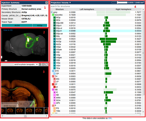
1. Injection Summary: This section includes a link to the Cortical Map Viewer from the icon in the top right-hand corner and lists the experiment ID, primary and secondary injection structure(s), the coordinates of the injection, the mouse strain, tracer type and the calculated injection summary (%) for the rAAV injection and the CAV injection (where appropriate). If the experiment was targeted stereotaxically, the coordinates are from a registration point (typically Bregma) in the anterior/posterior, dorsal/ventral, medial/lateral orientations and the angle of injection (AP, ML, DV, <). If the experiment was targeted using ISI, the coordinates will read “ISI(0, 0, DV, <)” indicating the depth and angle of injection (see Overview whitepaper in Documentation). If the experiment shown is from a transgenic line, you will also have a description of the infected cells and a link to the Transgenic Characterization of that line.
2. Projection Density Image Viewer: This viewer offers a rotating preview of the projection signal in 3 dimensions. Click the “View in 3D” link to view the experiment in the Brain Explorer software.
3. Section Images Viewer The Section Images viewer allows you to browse the experiment in 2-D. You can scroll through thumbnails of each section, zooming in or out and panning through areas of interest.
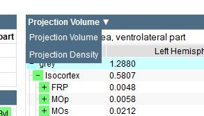
4. Histogram: This section illustrates the quantified signal in each structure either by projection volume (mm3) or by projection density (fraction of area occupied by signal compared to the whole structure). Toggle the two representations of the data using the drop down menu at the top of the histogram. The selected structure ontology can be expanded or collapsed and the number of structures shown can be changed using the threshold slider bar at the top of the histogram. When you click on a structure in the histogram, you will be taken to that area of the brain in the 3-D and 2-D image viewers. A red cross-hair pinpoints the center of that structure in each of the image viewers.
Data from this page can be downloaded as XML.
Experiment Image Viewer
To view several experiments in a single window, check the boxes next to experiments of interest from the various search methods. Once you have selected “View Selections” a window will open with all your checked experiments. The experiment image view displays images for each selected experiment in a Section Images viewer. This view makes it easy to compare experiments with each other and with the associated reference atlas, and with the Reference Data.
Multiple image series can be opened on the same page to enable side-by-side comparisons. Arrange the experiments by dragging an image viewer by the title bar and dropping into a new location. Add a reference atlas by selecting one from the “Atlases” drop-down menu in the upper-right hand corner of the window (see screenshot).
If you are viewing more than one experiment, open the configuration options to change the number of columns displayed in the window. The configuration options are accessible by clicking on the button with a “gear” icon to the right of the “Atlases” menu.
The injection site, section number and experiment ID are displayed in the title bar. Experiments using transgenic mice will also report the name of the transgenic line. Icons in the toolbar allow for you to take actions on the current image.
To view an overlay of each of the selected experiments in the Experiment Image Viewer, click on the Composite Projection Viewer in the title bar.
Using the Section Images Viewer
The Section Images Viewer is a powerful tool to navigate and view the images in an experiment. The main part of the viewer is an interactive window where an image can be repositioned by dragging with a mouse. Use the scroll wheel, on-screen navigation buttons or the keyboard to zoom in or out.
Thumbnails for the entire image series are displayed across the bottom of the viewer in section order. Click a thumbnail to select it for viewing, or use the keyboard to navigate through the set. The current selection is outlined in black.
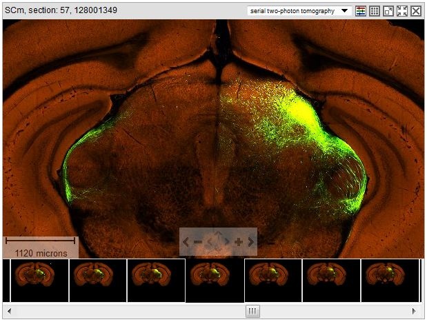
Scale Bar
Drag the scale bar with your mouse to the desired location. Click the scale bar text with your mouse to toggle between horizontal and vertical scale bars.
Using the Section Images Viewer Toolbar
Use the toolbar to take actions on the current image. Toolbar controls include:

Select between raw data and projection segmentation images

Adjust image controls
View all images in this experiment in a Contact Sheet Viewer

Synchronize all other section image viewers on the page that support synchronization to the currently selected image

Close the Section Images viewer
Keyboard Commands
Use the keyboard to navigate through the image series and synchronize the viewers on the page. Keyboard commands include:
You can also use the arrow keys to pan the current image.
Composite Projection Viewer
The Composite Projection Viewer allows you to see several projection experiments overlaid on the reference brain. This view allows you to sync experimental images with the reference atlas and other reference data.

The elements of this viewer include:
- Toggle between the individual image viewers and the composite viewer
- Add the coronal or sagittal reference atlas (will display below the Composite View) or change the number of columns (from the “gear”)
- The Composite View. Clicking the “+” in the top left-hand corner will open up images of each experiment
- Display reference data such as the annotated reference atlas or histochemical stains that was already in your viewing cart
Composite View
The composite view illustrates each selected experiment in an arbitrary color as circles based on the signal density in that voxel. Navigate the image viewer using the onscreen navigation tools or the options in the toolbar.
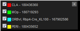
Composite View Toolbar

Choose your orientation - coronal, sagittal or horizontal

Change the size of the circle (0-3 Ergs)

Move through the sections with the slider bar (microns)

Sync composite image to the reference data

See selected experiments in the Brain Explorer 3-D Viewer
Contact Sheet Viewer
The contact sheet viewer shows serial sections of the selected experiment. Background fluorescence in the red channel illustrates basic anatomy and structures of the brain, and the injection site and projections are shown in the green channel.

High Resolution Image Viewer
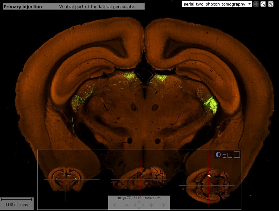
The High Resolution Image Viewer is launched from the contact sheet display or from clicking the icon in the Section Images Viewer and allows you a closer look at the image data.
The High Resolution Image Viewer consists of the main image viewer, a scale bar, and a multi-planar viewer. The primary injection site is listed in the title bar in the image viewer. The multi-planar viewer shows the three orthogonal views of the fluorescent projection; the coronal sections generated by two-photon tomography, and the sagittal and horizontal planes that were reconstructed from the coronal sections. Cross-hairs indicate the current location in the main viewer. Navigation of the main coronal image is via clicking on the planar views or by using the keyboard commands.
In the title bar are icons that allow you to interact with the main viewer.

A dropdown menu to view projection or segmentation images

Clicking on this icon will bring up a side by side synced view of the Interactive Atlas Viewer

Clicking on this icon will open a drop-down menu where you can; download an image, adjust the image controls, remove the title bar or remove the multiplanar viewer

The multiplanar viewer can be enlarged by clicking on the 3 varied sized boxes in the top-right corner of the viewer. Clicking on the circle in this toolbar toggles the transparency of the multiplanar viewer so that you can see the image in the main viewer behind the multiplanar viewer or not.
Keyboard Commands
In the High Resolution Image Viewer, use the keyboard commands to navigate through the image series to keep desired zoom and pan selections activated. Keyboard commands include:
You can also use the arrow keys to pan the current image.
Image Controls
When the “Color Adjustment…” is chosen from the tool icon drop-down menu, you will be presented with a window that allows you to adjust the dynamic range of each channel with a slider bar. What each color represents is outlined above each slider bar and you can exclude any of the channels by unchecking the box next to the slider bar. Once you have adjusted the properties of any channel, you can reset to the default settings by pressing the ‘Reset’ button.
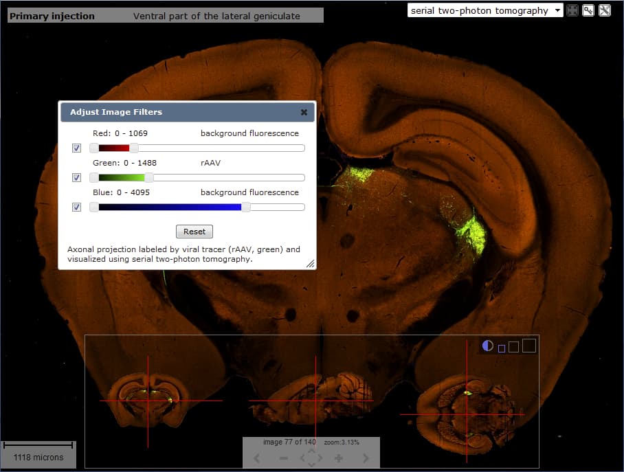
Each serial two-photon tomography image is stored as a three channel Red-Green-Blue (RGB) image with 16-bit per channel resolution. Since web browsers only support 8-bit viewing, we use intensity windowing to compress 16-bit data to 8-bit data. All pixel values below the specified minimum are displayed as black, pixel values above the specified maximum are displayed as green (or red/ blue depending on the channel). The pixel values in between are linearly stretched over the 8-bit range.
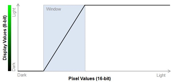
To make an image appear brighter, move the window sliders to the left, to make an image darker move the window sliders to the right. To increase contrast, move the sliders towards each other, to decrease contrast move the sliders away from each other.
The image below gives an example of how to brighten an image to enhance low intensity projections.
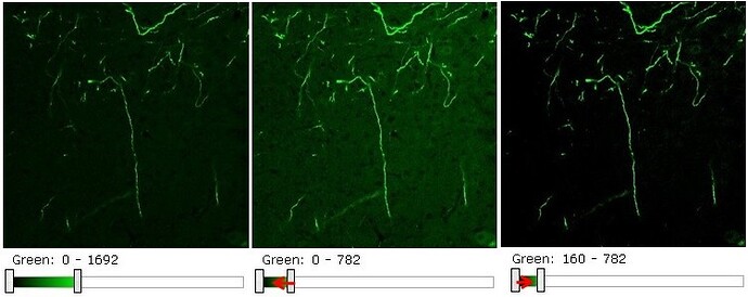
This next example shows how to darken and increase contrast of an image to look at details at the injection site. Note: turning on the blue channel may increase the resolution of individual cell-bodies at the site of infection.
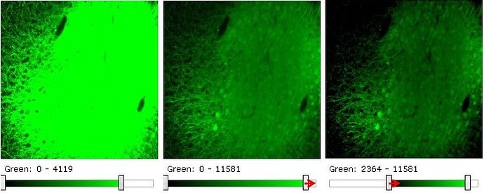
Note: the first three-quarters of the slider-bar represents the lower (0,4095) pixel value range in linear scale. The last quarter of the slider-bar represents the remaining upper (4096, 65535) range in log2 scale. The dual scaling allows for a compact representation of the full range, while allowing for fine-scale control at the lower end.
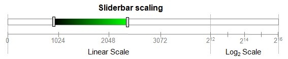
Learn about API Allen Brain Connectivity Atlas with comprehensive guides and examples from Allen Institute for Brain Science.
The primary data of the Allen Mouse Brain Connectivity Atlas consists of high-resolution images of axonal projections targeting different anatomic regions or various cell types using Cre-dependent specimens. Each data set is processed through an informatics data analysis pipeline to obtain spatially mapped quantified projection information.
From the API, you can:
Download Images
Download quantified projection values by structure
Download quantified projection values as 3-D grids
Query the source, target, spatial and correlative search services
Query the image synchronization service
Download atlas images, drawings and structure ontology
This document provides a brief overview of the data, database organization and example queries. API database object names are in camel case. See the main API documentation for more information on data models and query syntax.
Experimental Overview and Metadata
Experimental data from the Atlas is associated with the “Mouse Connectivity Projection” Product.
Each Specimen is injected with a viral tracer that labels axons by expressing a fluorescent protein. For each experiment, the injection site is analyzed and assigned a primary injection structure and, if applicable, a list of secondary injection structures.
Labeled axons are visualized using serial two-photon tomography. A typical SectionDataSet consists of 140 coronal images at 100 µm sampling density. Each image has 0.35 µm pixel resolution and raw data is in 16-bit per channel format. Background fluorescence in the red channel illustrates basic anatomy and structures of the brain, and the injection site and projections are shown in the green channel. No data was collected in the blue channel.
From the API, detailed information about SectionDataSets, SectionImages, Injections and TransgenicLines can be obtained using RMA queries.
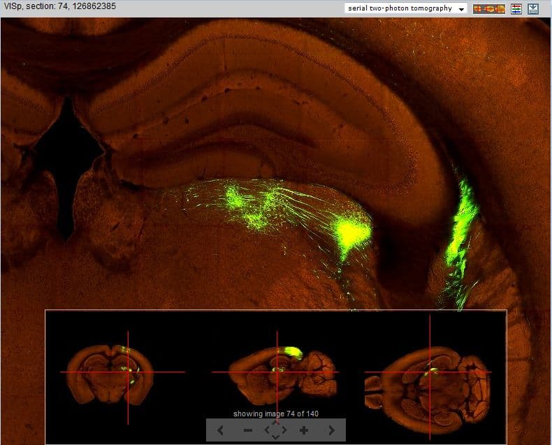
Figure: Projection dataset (id=126862385) with injection in the primary visual area (VISp) as visualized in the web application image viewer.
To provide a uniform look over all experiments, default window and level values were computed using intensity histograms. For each experiment, the upper threshold defaults to (2.33 x the 95th percentile value) for the red channel and (6.33 x the 95th percentile value) for the green channel. The default threshold can be used to download images and/or image region in 8-bit per channel image format.
In the web application, images from the experiment are visualized in an experimental detail page. All displayed information, images and structural projection values are also available through the API.
Informatics Data Processing
The informatics data processing pipeline produces results that enable navigation, analysis and visualization of the data. The pipeline consists of the following components:
- an annotated 3-D reference space,
- an alignment module,
- a projection detection module,
- a projection gridding module, and
- a structure unionizer module.
The output of the pipeline is quantified projection values at a grid voxel level and at a structure level according to the integrated reference atlas ontology. The grid level data are used downstream to provide a correlative search service and to support visualization of spatial relationships. See the informatics processing white paper for more details.
3-D Reference Models
The cornerstone of the automated pipeline is an annotated 3-D reference space. For this purpose, a next generation of the common coordinate framework (CCF v3) is being created based on an average population of 1675 specimens. See the Allen Mouse Common Coordinate Framework whitepaper for detailed construction information. In this current release, the framework consists of 207 newly drawn structures spanning approximately half the brain. To support whole brain quantification, structures which have not yet been drawn are extracted and merged from the version 2 framework based on the Allen Reference Atlas. The interfaces between old and new structures were manually inspected and filled to create smooth transitions to create a complete brain map (~700 structures) for quantification.

Structures in the common coordinate framework are arranged in a hierarchical organization. Each structure has one parent and denotes a “part-of” relationship. Structures are assigned a color to visually emphasize their hierarchical positions in the brain.
All SectionDataSets are registered to ReferenceSpace id = 9 in PIR orientation (+x = posterior, +y = inferior, +z = right).
3-D annotation volumes were updated in the October 2017 release to include newly drawn structures in the Allen Mouse Common Coordinate Framework (CCFv3).
Volumetric data files available download:
Each data type is available in multiple voxel resolutions:
All volumetric data is compressed NRRD (Nearly Raw Raster Data) format. The raw numerical data is stored as a 1-D array raster as shown in the figure below.
Example Matlab code snippet to read in the 25µm template and annotation volumes:
% -------------------------------
%% Download a NRRD reader
% For example:
% http://www.mathworks.com/matlabcentral/fileexchange/50830-nrrd-format-file-reader
%
% Requires: MATLAB 7.13 (R2011b)
%
% Download:
%   average_template_25.nrrd
%   ara_nissl_25.nrrd
%   ccf_2015/annotation_25.nrrd
% -------------------------------

%% Read image volume with NRRD reader
% Note: reader swaps the order of the first two axes
%
% AVGT  = 3-D matrix of average_template
% NISSL = 3-D matrix of ara_nissl
% ANO   = 3-D matrix of ccf_2015/annotation

[AVGT, metaAVGT] = nrrdread('average_template_25.nrrd');
[NISSL, metaNISSL] = nrrdread('ara_nissl_25.nrrd');
[ANO, metaANO] = nrrdread('annotation_25.nrrd');

%% Display one coronal section
figure;
imagesc(squeeze(AVGT(:, 264, :)));
colormap(gray(256));
axis equal;

figure;
imagesc(squeeze(NISSL(:, 264, :)));
colormap(gray(256));
axis equal;

figure;
imagesc(squeeze(ANO(:, 264, :)));
caxis([1, 2000]);
colormap(lines(256));
axis equal;

%% Display one sagittal section
figure;
imagesc(squeeze(AVGT(:, :, 220)));
colormap(gray(256));
axis equal;

figure;
imagesc(squeeze(NISSL(:, :, 220)));
colormap(gray(256));
axis equal;

figure;
imagesc(squeeze(ANO(:, :, 220)));
caxis([1, 2000]);
colormap(lines(256));
axis equal;
Example Python code snippet to read in the 25µm template and annotation volumes:
# -------------------------------
# Install pynrrd:
# https://github.com/mhe/pynrrd
#
# Download:
#   average_template_25.nrrd
#   ara_nissl_25.nrrd
#   ccf_2015/annotation_25.nrrd
# -------------------------------

import nrrd
import numpy as np
import matplotlib.pyplot as plt
from PIL import Image

# ---------------------------------
# Read image volume with NRRD reader
# Note: reader swaps the order of the first two axes
#
# AVGT  = 3-D matrix of average_template
# NISSL = 3-D matrix of ara_nissl
# ANO   = 3-D matrix of ccf_2015/annotation
# ---------------------------------

AVGT, metaAVGT = nrrd.read('average_template_25.nrrd')
NISSL, metaNISSL = nrrd.read('ara_nissl_25.nrrd')
ANO, metaANO = nrrd.read('annotation_25.nrrd')

# ---------------------------------
# Save one coronal section as PNG
# ---------------------------------
slice = AVGT[264, :, :].astype(float)
slice /= np.max(slice)
im = Image.fromarray(np.uint8(plt.cm.gray(slice) * 255))
im.save('output/avgt_coronal.png')

slice = NISSL[264, :, :].astype(float)
slice /= np.max(slice)
im = Image.fromarray(np.uint8(plt.cm.gray(slice) * 255))
im.save('output/nissl_coronal.png')

slice = ANO[264, :, :].astype(float)
slice /= 2000
im = Image.fromarray(np.uint8(plt.cm.jet(slice) * 255))
im.save('output/ano_coronal.png')

# ---------------------------------
# Save one sagittal section as PNG
# ---------------------------------
slice = AVGT[:, :, 220].astype(float)
slice /= np.max(slice)
im = Image.fromarray(np.uint8(plt.cm.gray(slice) * 255))
im.save('output/avgt_sagittal.png')

slice = NISSL[:, :, 220].astype(float)
slice /= np.max(slice)
im = Image.fromarray(np.uint8(plt.cm.gray(slice) * 255))
im.save('output/nissl_sagittal.png')

slice = ANO[:, :, 220].astype(float)
slice /= 2000
im = Image.fromarray(np.uint8(plt.cm.jet(slice) * 255))
im.save('output/ano_sagittal.png')
Image Alignment
The aim of image alignment is to establish a mapping from each SectionImage to the 3-D reference space. The module reconstructs a 3-D Specimen volume from its constituent SectionImages and registers the volume to the 3-D reference model by maximizing mutual information between the red channel of the experimental data and the average template.
Once registration is achieved, information from the 3-D reference model can be transferred to the reconstructed Specimen and vice versa. The resulting transform information is stored in the database. Each SectionImage has an Alignment2d object that represents the 2-D affine transform between an image pixel position and a location in the Specimen volume. Each SectionDataSet has an Alignment3d object that represents the 3-D affine transform between a location in the Specimen volume and a point in the 3-D reference model. Spatial correspondence between any two SectionDataSets from different Specimens can be established by composing these transforms.
For convenience, a set of “Image Sync” API methods is available to find corresponding positions between SectionDataSets, the 3-D reference model and structures. Note that all locations on SectionImages are reported in pixel coordinates and all locations in 3-D ReferenceSpaces are reported in microns. These methods are used by the Web application to provide the image synchronization feature in the multiple image viewer (see Figure).
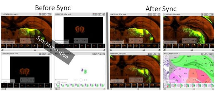
Projection Data Segmentation
For every Projection image, a grayscale mask is generated that identifies pixels corresponding to labeled axon trajectories. The segmentation algorithm is based on image edge/line detection and morphological filtering.
The segmentation mask image is the same size and pixel resolution as the primary projection image and can be downloaded through the image download service.

Reference-aligned Image Channel Volumes
The red, green, and blue channels have been aligned to the 25um adult mouse brain reference space volume. These volumes have been stored in the API WellKnownFile table with type name “ImagesResampledTo25MicronARA”. To retrieve the download link for a specific data set, query for WellKnownFiles of the appropriate type with an “attachable_id” equal to the data set id:
http://api.brain-map.org/api/v2/data/WellKnownFile/query.xml?criteria=well_known_file_type[name$eq’ImagesResampledTo25MicronARA’][attachable_id$eq156198187]
Download this by attaching the value of the download-link field to the API web host name (http://api.brain-map.org/api/v2/well_known_file_download/269830017). The download file will be a .zip file containing three images stored in the raw meta image format:
- resampled_red.mhd/raw: red background fluorescence
- resampled_green.mhd/raw: rAAV signal
- resampled_blue.mhd/raw: blue background fluorescence
All volumes have the same dimensions as the 25um adult mouse reference space volume.
Projection Data Gridding
For each dataset, the gridding module creates a low resolution 3-D summary of the labeled axonal trajectories and resamples the data to the common coordinate space of the 3-D reference model. Casting all data into a canonical space allows for easy cross-comparison between datasets. The projection data grids can also be viewed directly as 3-D volumes or used for analysis (i.e. target, spatial and correlative searches).
Each image in a dataset is divided into a 10 x 10 µm grid. In each division, the sum of the number of detected pixels and the sum of detected pixel intensity were collected. A second set of these same summations was computed for the regions manually identified as belonging to the injection site for injection site quantification. The resulting 3-D grid is then transformed into the standard reference space using linear interpolation to generate sub-grid values.
From the summations we obtained measures for:
- projection density = sum of detected pixels / sum of all pixels in division
- projection energy = sum of detected pixel intensity / sum of all pixels in division
- injection_fraction = fraction of pixels belonging to manually annotated injection site
- injection_density = density of detected pixels within the manually annotated injection site
- injection_energy = energy of detected pixels within the manually annotated injection site
- data_mask = binary mask indicating if a voxel contains valid data (0=invalid, 1=valid). Only valid voxels should be used for analysis
For each summation type, grid files can be downloaded at 10, 25, 50 and 100 μm isotropic voxel resolution.
3-D grids were updated in the May 2015 release to reflect the remapping to the new Allen Mouse Common Coordinate Framework (CCFv3), higher resolution computation and a new compress data format. 3-D grids from the October 2014 release (mapped to CCFv2) can be accessed through our data download server (see instructions).
Grid data for each SectionDataSet can be downloaded using the 3-D Grid Data Service. The service returns a compressed NRRD (Nearly Raw Raster Data) 32-bit FLOAT format. To download a particular grid file, the user specifies the SectionDataSet ID, the type of grid and the resolution.
Examples:
- Download projection_density for a VISal injection SectionDataSet (id=287495026) at 50 μm resolution
http://api.brain-map.org/grid_data/download_file/287495026??image=projection_density&resolution=50
Example Matlab code snippet to read in the 50 µm projection_density grid volume and average_template:
% -------------------------------

%

% Download a NRRD reader

% For example:

% http: //www.mathworks.com/matlabcentral/fileexchange/50830-nrrd-format-file-reader

%

% Requires: MATLAB  7.13 (R2011b)

%

% Download average_template_50.nrrd

% Download projection_density at  50 micron  for SectionDataSet id =  287495026

%

% ---------------------------------

%

% Read image volume with NRRD reader

% Note that reader swaps the order of the first two axes

%

% AVGT =  3 -D matrix of average_template

% PDENS =  3 -D matrix of projection_density

% DMASK =  3 -D matrix of data_mask

%

[AVGT, metaAVGT] = nrrdread( 'average_template_50.nrrd' );

[PDENS, metaPDENS] = nrrdread( '11_wks_coronal_287495026_50um_projection_density.nrrd' );

[DMASK, metaDMASK] = nrrdread( '11_wks_coronal_287495026_50um_data_mask.nrrd' );

% Display one coronal section

figure;imagesc(squeeze(AVGT(:, 184 ,:)));colormap(gray( 256 )); axis equal;

figure;imagesc(squeeze(PDENS(:, 184 ,:)));colormap(jet( 256 )); axis equal;

figure;imagesc(squeeze(DMASK(:, 184 ,:)));colormap(gray( 256 )); axis equal;
Example Python code snippet to read in the 50 µm injection_density and injection_fraction and compute an injection centroid:
# -------------------------------

#

# Install pynrrd: https: //github.com/mhe/pynrrd

#

# Download injection_density at  50 micron  for SectionDataSet id =  287495026

# Download injection_fraction at  50 micron  for SectionDataSet id =  287495026

#

# ---------------------------------

import nrrd

import numpy as np

import matplotlib.pyplot as plt

import Image

#

# Read image volume with NRRD reader

# Note that reader swaps the order of the first two axes

#

# INJDENS =  3 -D matrix of injection_density

# INJFRAC =  3 -D matrix of injection_fraction

#

INJDENS, metaINJDENS = nrrd.read( '11_wks_coronal_287495026_50um_projection_density.nrrd' );

INJFRAC, metaINJFRAC = nrrd.read( '11_wks_coronal_287495026_50um_injection_fraction.nrrd' );

# find all voxels with injection_fraction >=  1

injection_voxels = np.where( INJFRAC >=  1 )

injection_density = INJDENS[injection_voxels]

sum_density = sum(injection_density)

# compute centroid in CCF coordinates

centroid = map( lambda x : sum( injection_density * x ) / sum_density *  50 , injection_voxels)

print centroid
Projection Structure Unionization
Projection signal statistics can be computed for each structure delineated in the reference atlas by combining or unionizing grid voxels with the same 3-D structural label. While the reference atlas is typically annotated at the lowest level of the ontology tree, statistics at upper level structures can be obtained by combining measurements of the hierarchical children to obtain statistics for the parent structure. The unionization process also separates out the left versus right hemisphere contributions as well as the injection versus non-injection components.
Projection statistics are encapsulated as a ProjectionStructureUnionize object associated with one Structure, either left, right or both Hemispheres and one SectionDataSet. ProjectionStructureUnionize can be downloaded via RMA. ProjectionStructureUnionize data is used in the web application to display projection summary bar graphs.
Examples:
http://api.brain-map.org/api/v2/data/ProjectionStructureUnionize/query.xml?criteria=[section_data_set_id$eq126862385], [is_injection$eqfalse]&num_rows=5000&include=structure
http://api.brain-map.org/api/v2/data/ProjectionStructureUnionize/query.xml?criteria=[section_data_set_id$eq126862385], [is_injection$eqtrue]&num_rows=5000&include=structure
Projection Grid Search Service
A projection grid service has been implemented to allow users to instantly search over the whole dataset to find experiments with specific projection profiles.
- The Source Search function retrieves experiments by anatomical location of the injection site.
- The Target Search function returns a rank list of experiments by signal volume in the user specified target structure(s).
- The Spatial Search function returns a rank list of experiments by density of signal in the user specified target voxel location.
- The Injection Coordinate Search function returns a rank list of experiments by distance of their injection site to a user specified seed location.
- The Correlation Search function enables the user to find experiments that have a similar spatial projection profile to a seed experiment when compared over a user-specified domain.
The projection grid search service is available through both the Web application and API.
Source Search
To perform a Source Search, a user specifies a set of source structures. The service returns all experiments for which either the primary injection structure or one of its secondary injection structures corresponding to one of the specified source structures or their descendents in the ontology. The search results can also be filtered by a list of transgenic lines.
See the connected service page for definitions of service::mouse_connectivity_injection_structure parameters.
The output of the source search is a xml list of objects. Each object represents one experiment and contains information about the experiment including its unique identifier, the primary injection structure, list of any secondary injection structures, injection coordinates, injection volume and transgenic line name.
Examples:
- Source search for experiments with injection in the isocortex
http://api.brain-map.org/api/v2/data/query.json?criteria= service::mouse_connectivity_injection_structure[injection_structures$eqIsocortex][primary_structure_only$eqtrue]
- Source search for experiments performed on wild-type specimens and with injection in the isocortex
http://api.brain-map.org/api/v2/data/query.json?criteria= service::mouse_connectivity_injection_structure[injection_structures$eqIsocortex][transgenic_lines$eq0][primary_structure_only$eqtrue]
- Source search for experiments performed on Syt6-Cre_KI148 cre-line specimens and with injection in the isocortex
http://api.brain-map.org/api/v2/data/query.json?criteria= service::mouse_connectivity_injection_structure[injection_structures$eqIsocortex][transgenic_lines$eq’Syt6-Cre_KI148’][primary_structure_only$eqtrue]

Target Search
To perform a Target Search, the user specifies a set of target structures. The service returns a rank list of experiments by signal volume in the target structures which are above a minimum threshold. The target structure specification can be further refined by hemisphere. The search results can also be filtered by a list of source structures and/or list of transgenic lines.
See the connected service page for definitions of service::mouse_connectivity_injection_structure parameters.
The output of the target search is a xml list of objects. Each object represents one experiment and contains information about the experiment including its unique identifier, the primary injection structure, list of any secondary injection structures, injection coordinates, injection volume and transgenic line name. Additionally, the total signal volume and number of voxels spanned by the target structure(s) is also reported.
Example:
- Target search for experiments with projection signal in the target structure LGd (dorsal part of the lateral geniculate complex) and injection in the isocortex
http://api.brain-map.org/api/v2/data/query.json?criteria= service::mouse_connectivity_injection_structure[injection_structures$eqIsocortex][primary_structure_only$eqtrue][target_domain$eqLGd]
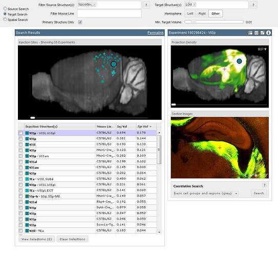
Spatial Search
To perform a Spatial Search, a user selects a target location within the 3D reference space. The service returns a rank list of experiments by signal density in the target location and with density greater than 0.1.
See the connected service page for definitions of service::mouse_connectivity_target_spatial parameters.
The output of the target search is a xml list of objects. Each object represents one experiment and contains information about the experiment including its unique identifier, the primary injection structure, list of any secondary injection structures, injection coordinates, injection volume and transgenic line name. Additionally, the path from the target location to the injection site is listed along with signal density at each node.
Example:
- Spatial search for experiments with projection signal in a target location in VM (ventral medial nucleus of the thalamus)
http://api.brain-map.org/api/v2/data/query.xml?criteria= service::mouse_connectivity_target_spatial[seed_point$eq6900,5050,6450]

Injection Coordinate Search
To perform an Injection Coordinate Search, a user specifies a seed location within the 3D reference space. The service returns a rank list of experiments by distance of its injection site to the specified seed location.
See the connected service page for definitions of service::mouse_connectivity_injection_coordinate parameters.
The output of the injection coordinate search is a xml list of objects. Each object represents one experiment and contains information about the experiment including its unique identifier, the primary injection structure, list of any secondary injection structures, injection coordinates, injection volume and transgenic line name. Additionally, distance between the injection site and seed location is also reported.
Example: Injection coordinate search for experiments with a seed location in VM (ventral medial nucleus of the thalamus)
http://api.brain-map.org/api/v2/data/query.xml?criteria= service::mouse_connectivity_injection_coordinate[seed_point$eq6900,5050,6450]
Correlation Search
To perform a Correlation Search, the user selects a seed experiment and a domain over which the similarity comparison is to be made. All voxels belonging to any of the domain structures form the domain voxel set. Pearson’s correlation coefficient is computed between the domain voxel set from the seed experiment and every other experiment in the product. The return list is sorted by descending correlation coefficient.
See the connected service page for definitions of service::service::mouse_connectivity_correlation parameters.
The output of the injection coordinate search is a xml list of objects. Each object represents one experiment and contains information about the experiment including its unique identifier, the primary injection structure, list of any secondary injection structures, injection coordinates, injection volume and transgenic line name. Additionally, the Pearson’s correlation coefficient between the experiment and the seed is reported.
Example:
- Correlation search for experiment with similar projection profile in the thalamus compared to seed experiment 112670853 (injection in primary motor area of the cortex)
http://api.brain-map.org/api/v2/data/query.xml?criteria= service::mouse_connectivity_correlation[row$eq112670853][structures$eqTH]

Learn about Transgenic Characterization with comprehensive guides and examples from Allen Institute for Brain Science.
From this tab you can browse and select from reporter lines and driver lines used in the creation of the Allen Mouse Brain Connectivity Atlas.
Searching
Search the Transgenic Mouse dataset by entering a gene symbol or mouse line name into the search box. Retinal Projectome data includes four experiments with vertical mount sections of the retina. You will be prompted with suggestions once you have started typing. Click “Search” or hit the Enter key.
You can also browse through the data using tabs on the search page that illustrate all of the Driver Lines and Reporter Lines used in this resource.
Driver Lines
Each driver line is represented by its name, a representative image (which is magnified when clicked) and a description of expression. Clicking on the line name will return results from all characterization experiments for that particular line.

Reporter Lines
This tab lists all the characterized reporter lines with a description of their expression patterns.
Retinal Projectome
Representative retinas were sectioned in the vertical plane for characterization of morphology and co-localization with markers for well defined retinal ganglion cell (RGC) types. Four markers were used:
- VAChT (vesicular acetylcholine transporter) - a marker of inner plexiform layers,
- CART (cocaine-amphetamine related transcript) - a marker of ON/OFF direction selective retinal ganglion cells,
- OPN osteopontin - a marker of large/ dephosphorylated neurofilament-positive RGCs,
- Brn3a which labels ~80% of all RGCs and is a Pit/Oct/Unc (POU) domain transcription factor.
Each experiment shows the GFP viral tracer infection in green, the marker in red and a DAPI stain in blue.
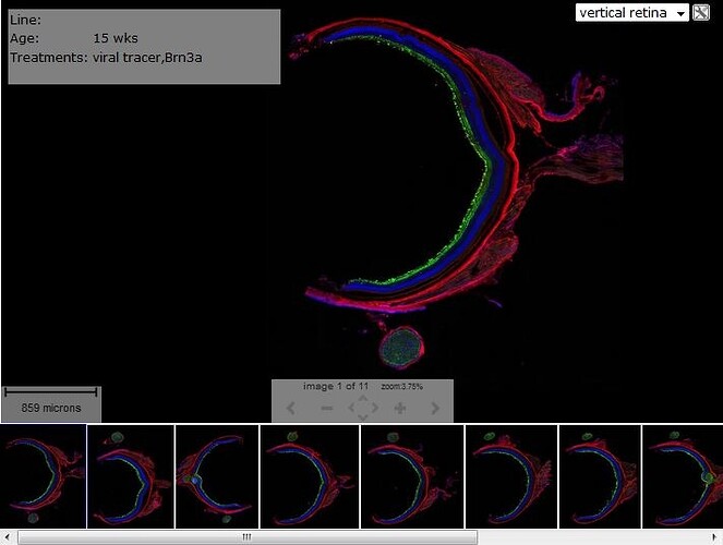
Search Results
Clicking on Search will return a list of experiments based on your search criteria with information on the Experiment ID, Line Name, Driver, Reporter, Probes, Age, Sex, Treatments and Image Count. Click on the Experiment ID to be taken to the Experiment Detail Page
To compare multiple experiments, mark the checkboxes to the left of each row, then click the “Compare Selected Experiments” button. Note: the selection list may contain previously selected experiments from the “Projection” or “BDA/AAV” studies. Your choices are stored in a browser ‘cookie’ on your computer and will remain in effect until you click the “Clear Selections” button, or clear your Web browser cookie cache.
Experiment Detail Page
Clicking on the experiment summary link returns a summary of the experimental details (see screenshot).
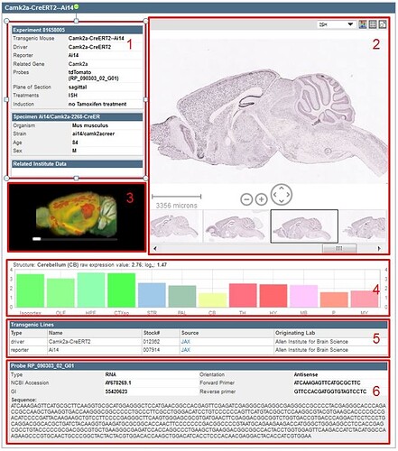
The various sections of the experimental detail page are outlined 1-6 as follows:
- Experimental Metadata: Experiment ID, Transgenic Mouse, Driver, Reporter, Related Gene (click for Adult Mouse data), Probes, Plane of Section, Treatments, Induction; Specimen Data: Specimen ID, Organism, Strain, Age, Sex. Related Institute Data: provides links to related data in other Allen Brain Atlas resources
- Image Viewer : Zoom and Pan Viewer
- 3D Thumbnail Viewer: Rotate using the slider bar under the image
- Histogram: Relative gene expression in large structures of the brain (for stages older than P28). Hovering your mouse over the histogram will sync the image in the single image viewer with the section corresponding to that structure and expression.
- Transgenic Line Metadata: Transgenic lines involved in this experiment including the Type, Name, Stock #, Source (link to provider), and the Originating Lab.
- Probe Information: Probe ID, Type, NCBI Accession, GI, Orientation, Forward Primer, Reverse Primer and Sequence.
Using the Zoom And Pan (ZAP) Image Viewer
The Zoom and Pan (ZAP) Image Viewer is a powerful tool to navigate and view the images in an experiment. The main part of the viewer is an interactive window where an image can be repositioned by dragging with a mouse. Use the scroll wheel, on-screen navigation buttons or the keyboard commands to zoom in or out.
Select other images in the experiment by clicking on a thumbnail image below the main viewer.
Scale Bar
Drag the scale bar with your mouse to the desired location. Click the scale bar text with your mouse to toggle between horizontal and vertical.
Using the ZAP Viewer Toolbar
Use the toolbar to take actions on the image that currently has focus. Toolbar controls include:
Select ISH, Nissl or Expression Energy
Image adjust controls
Display all thumbnail images in a single contact sheet

Open the selected image in the High Resolution Image Viewer
Keyboard Commands
Use the keyboard to navigate through the image series and synchronize the viewers on the page. Keyboard commands include:
You can also use the arrow keys to pan the current image.
Expression Energy
The expression mask image display highlights those cells that have the highest probability of gene expression using a heat map color scale (from low/blue to high/red).
The Expression Energy was calculated as follows: Within a given area A (voxel or structure), expression energy = (sum of intensity of expressing pixels in A) / (sum of all pixels in A):
Learn about Reference Data Mouse Connectivity with comprehensive guides and examples from Allen Institute for Brain Science.
From this tab you can browse from a list of 5 reference dataset experiments. This datasets are also available to add to the cart so you can view them simultaneously with the Projection, BDA vs. rAAV and Transgenic datasets. To select a dataset, click the checkbox and then click “View Selections”. These selections will be stored as a “cookie” in your browser until you click the “Clear Selections” button.
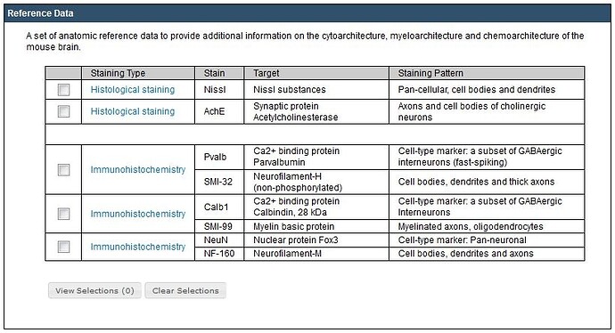
ach reference dataset outlines the stain, the target of the stain as well as the staining pattern. Selecting a reference dataset will return the experiment ID, Mouse Strain, Sex, and Age.
Viewing the Experiments
Clicking on the experiment ID will launch a contact sheet viewer. Double-click an individual image in the contact sheet viewer to launch a High Resolution Image Viewer. The experiment ID, stains and section number are listed on the title banner of the viewer. Navigate through the images via the navigation panel in the main image viewer, or use the Keyboard Commands. To download the image, click the icon (see below).


To adjust the image filters, click on the icon in the top right-hand corner of the viewer. The stains used in each channel are listed on the image filter adjustment tool. To turn off a channel, unclick the checkbox next to that channel. Moving the slider bars to the left will decrease the brightness of that channel, while moving the slider bars to the right will increase the channel brightness. Click the reset button to set to default levels.
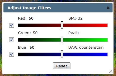
Keyboard Commands
In the High Resolution Image Viewer, use the keyboard commands to navigate through the image series. Keyboard commands include:
You can also use the arrow keys to pan the current image.
Learn about Brain Explorer 3d Viewer with comprehensive guides and examples from Allen Institute for Brain Science.
Brain Explorer® 3-D Viewer is an application for viewing brain anatomy, gene expression and fluorescence projection data in three dimensions in the framework of the Allen Reference Atlas.
Using Brain Explorer, you can:
• View a fully interactive version of the Allen Reference Atlas in 3-D.
• View gene expression data in 3-D at 200 µm3 resolution.
• View projection data in 3-D at 100 µm3 resolution.
• View expression data and projection data from multiple experiments superimposed on each other in 3-D.
• Navigate the high-resolution 2-D ISH and projection images using the 3-D model.
• Link to associated gene metadata on the Allen Mouse Brain Atlas web application.
Installation
Windows
Systems requirement: minimum configuration
• Operating System: Microsoft Windows 7
• CPU: Intel Core Duo or AMD 1.8GHz
• System Memory: 1GB
• Graphics Card: Hardware 3D OpenGL accelerated AGP or PCI Express with 64MB RAM
• Screen: 1024x768, 32-bit true color
• Hard Disk: 200MB free space
Note: Brain Explorer is known to work with the following video chipsets: nVidia GeForce 9400/9600, nVidia Quadro FX 1800/3800/5600, AMD Radeon 9600, AMD Radeon HD 3200/4550, Intel Q35/Q45 Express.
For the best performance, please check with your video card vendor for the latest available drivers before using Brain Explorer. The Windows version of the Brain Explorer viewer is available here. Double-click the downloaded BrainExplorer2.msi file and follow the prompts.
Mac
Systems requirement: minimum configuration
• Operating System: OS X 10.6.8
• CPU: Intel 1.8GHz
• System Memory: 1GB
• Graphics Card: 3D-capable with 64MB RAM
• Screen: 1024x768, 32-bit millions of colors
• Hard Disk: 200MB free space
Note: Please install the latest system updates from Apple to ensure you have the latest video card drivers.
The Mac version of the Brain Explorer viewer is available here. Double-click the downloaded zip file to unpack Brain Explorer.
Installing Atlases
A one-time download containing anatomy files is needed following installation of the Brain Explorer application. The first time you open the Brain Explorer software, you will be asked to choose to download files for the Allen Developing Mouse and Allen Human Brain atlases. Click on the atlases you would like to use and then click the Install button.
To download missing atlases on the PC, go to the Help menu and select Download Atlases. On the Mac, the command is in the Brain Explorer 2 menu.
Getting Updates
The Brain Explorer application will inform you when updates to the Brain Explorer application itself or its atlases are available. New data may not be available for viewing until you install the required updates.
Viewing Projection Data
To load projection data into the Brain Explorer viewer, go to the Allen Mouse Brain Connectivity Atlas and perform an efferent search. You can also select a structure name from the list of injection sites. Your search brings back a list of experiments. Click on a row to select an experiment of interest. A 3-D thumbnail of the projection data of that experiment will appear to the right. Click on the blue “View in 3D” file link to launch the Brain Explorer application.

When the Brain Explorer 3-D Viewer opens, you will be taken to a screen that displays the Image Viewer, the Structure Ontology Viewer, and the Gene/Projection List.
Image Viewer
The Image Viewer displays a 3-D representation of the neuronal projections in the selected experiment. Each sphere (when present) represents the injection site re-sampled to a 100 micron grid resolution. Each line traces fluorescent signal through the brain and each cube represents termination of signal. Larger polygons corresponds to a greater density of signal. Gene expression data can be displayed concurrently with the projection data. Gene expression will also be represented by spheres as described in here.
You can select a sphere or cube by clicking on it. Volumes can be deselected by clicking on blank space. The original projection section of the selected sphere/cube will be displayed blended with the projection segmentation in the lower left hand portion of the screen. The blending can be adjusted by selecting Image Controls from the View menu and moving the Image Blending slider. Clicking on the arrow in the projection image will open the corresponding image in a high resolution image viewer.
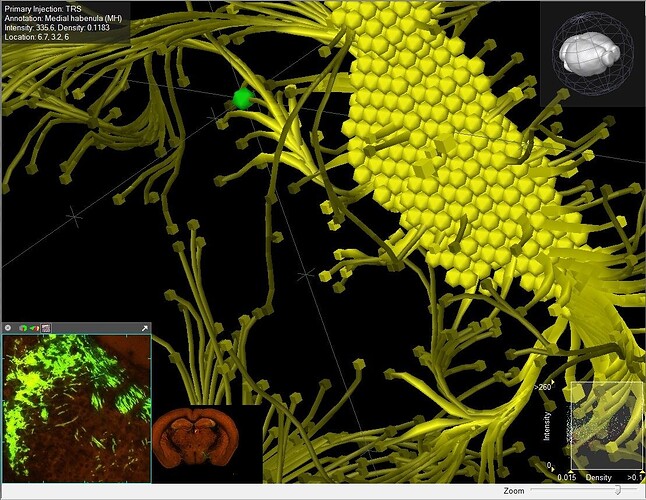
The information at the upper left corner of the main Brain Explorer window summarizes the fluorescent signal detected in the selected grid location. This information includes the primary injection site, the annotated location of the selected point, average signal density and intensity (over pixels) and the location. The Informatics Data Processing White Paper describes how the measurements were obtained.
To change the projection signal representation, click on the “Data” tab in the top left hand corner of your screen and select an option under “Raw” colors.
A compass in the right-hand corner of the Image Viewer can be used to rotate the brain by clicking and dragging your cursor. You can zoom using either the wheel on your mouse or using the Zoom scrollbar in the lower right hand corner of the Image Viewer.
Projection Thresholds
A way to control projection visibility is by setting thresholds on projection signal values. This method can restrict visible signals to different combinations such as low intensity and low density or high intensity and low density.
The graph in the lower right hand corner shows a dot for each streamline endpoint, shown as a cube, in a projection experiment. The color of the dot corresponds to the anatomic annotation in the same way the atlas colors display mode works. Each data point is plotted according to its density on the x-axis and its intensity on the y-axis.
The thresholds can be changed by resizing the white box. Any edge or corner of the box can be clicked and dragged to re-size it. You can also click and drag in the center of the box to move the box.
Structure Ontology Viewer
The Structure Ontology Viewer shows the entire collapsible ontology for the mouse brain as defined by the Allen Reference Atlas. Two columns to the right of the ontology determine the type of data displayed in the Image Viewer. “A” represents annotation and when checked, will show a visual representation of that structure in the Image Viewer. “D” represents signal density and when checked, will show signal in that structural domain.
The default organization for the Structure Ontology is the Hierarchical View, but if you are unfamiliar with the ontology, you can click on the Alphabetical View to see the structure list in alphabetical order.
The Bookmarks tab is a space where you can create and save favorite views of the brain. Several default views are already saved that will rotate the brain back into common viewing frames.
Gene/Projection List
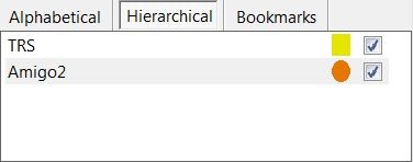
This section displays projection experiments you have selected as well as any gene expression experiments you have downloaded in this session. Projection data is indicated by a colored square, gene expression by a colored circle. Right clicking on the gene name or injection site will bring up a menu where you can, 1) view the gene or experiment detail page (Get Info), 2) be taken to a zoomed in image from this experiment (View Images), 3) copy meta information to the clipboard, such as symbol, name, Entrez ID, image-series ID (Copy Info), 4) activate a “Find Correlates” search finding experiments with similar profiles (Find Similar) or 5) close the experiment and remove it from the list and the 3-D view (Close).
Gene Search
To search for genes within the Brain Explorer application: go to the Search box located above the ontology panel and type in the gene symbol or part of a gene name.
The list of results shows gene name, gene symbol along with a 3-D summary thumbnail of the expression for each experiment matching the search. The expression thumbnail represents a maximum expression projection rendering: the denser the expression in a region the more “solid” the appearance. Reference atlas colors are additionally layered on top.
To load an experiment for viewing click on the “Download” button under the gene name.
Toolbar

: Selects cursor rotation tool mode

: Selects cursor pan tool mode

: Selects cursor selection tool mode

: Toggle Sagittal Atlas section viewing

: Toggle Coronal Atlas section viewing

: Toggle Horizontal Atlas section viewing

: Centers the Viewer on the current pinpointed expression data point

: Turns on the cutting planes

: Toggles the Structure Ontology and Gene List View
Advanced Features
Atlas Tab:
You can show opaque three dimensional structures of the brain by “showing” or “hiding” structures from this menu. The “Transparent” function allows you to see transparent views of the structures to view the anatomical relationships between them.
Selecting the sagittal, coronal or horizontal sections (or clicking on one of the section image buttons in the toolbar) will superimpose a single plane of the Nissl images from each brain on your image space. These planes can be moved once the selection tool mode button in the toolbar is selected. Selecting “Show Annotation on Section” from this menu will color the Nissl images according to the brain structure ontology.
Select “Show Full Resolution Image” to link to the high resolution annotation reference atlas images.
Data Tab:
The Data Tab menu allows to you to show all signal, hide all signal (for instance to then select a single structure) or toggle expression (for instance, unselect your region of interest then toggle to see signal in only that region).
You can also show or remove threshold controls and choose the visual representation of your data from this menu. There are several options under “Raw” colors:
- User defined: each experiment is rendered in user specified color. This mode is useful to distinguish between individual experiments when multiple experiments are being displayed.
- Atlas: In this mode the signal is colored by the corresponding reference atlas structure color. This mode is useful for quickly seeing the annotated regions where a fluorescent signal is detected.
- Signal Level: this mode display average signal intensity and is useful for identifying areas of very high signal.
To be taken to the experiment contact sheet page, select “Get Info”. To see a high resolution view of the images in this experiment choose “View Images”. These functions are also available by right-clicking on the injection site/gene name in the Gene/Projection List.
Choose “Find Similar” to find similar experiments to the selected experiment. This uses the same NeuroBlast functionality as in the web application.
Clipping Planes:
When this function is selected, either by toggling the cutting tools button in the toolbar or selecting “Clipping Planes” from the View drop down menu, you can make coronal, sagittal or horizontal cuts in your view of the brain and related data. To cut in a particular plane, make sure the cursor is in selection tool mode, and then click and drag on the plane you are interested in clipping.
Troubleshooting
Windows
Graphics
If you are using a desktop computer, you should obtain drivers from the video card manufacturer. First, identify the video card. Go the Start menu and open the Control Panel. Open the Display control panel and go to the Settings tab. Click the Advanced button and go to the Adapter tab. Your video card vendor and model name will be displayed at the top of the window under Adapter Type. Please go to the manufacturer’s web site, locate the driver download, and follow the instructions on the website or included with the downloaded file.
If you are using a laptop computer, you will need to go to your laptop manufacturer’s web site to locate the latest video drivers.
You can also activate an alternate drawing mode in Brain Explorer. Go to the View menu and select Options. Check the Draw faster but at lower quality button and uncheck the Synchronize drawing with the monitor’s vertical refresh button. Set the Multisample setting to Off.
If you are using multiple video cards from different vendors, the 3-D display may not work correctly on all attached monitors.
Uninstalling
Use the Add/Remove Programs control panel or the uninstall link in the Brain Explorer folder in the Start menu. Additional data that are not automatically uninstalled are located at the following locations:
Windows XP
Atlas data: C:\Documents and Settings\userid\Local Settings\Application Data\Allen Institute\Brain Explorer 2
User settings: C:\Documents and Settings\userid\Application Data\Allen Institute\Brain Explorer 2
Windows Vista and Windows 7
Atlas data: C:\Users\userid\AppData\Local\Allen Institute\Brain Explorer 2
User settings: C:\Users\userid\AppData\Roaming\Allen Institute\Brain Explorer 2
Proxy Settings
If you use a proxy server, the Brain Explorer application will use the proxy settings from the Internet Options control panel in the Windows Start menu. Please refer to the Windows documentation for help on proxy settings.
Mac
Uninstalling
Drag the Brain Explorer 2 icon to the trash. The Brain Explorer application generates the following files, which can also be dragged to the trash.
- ~/Library/Application Support/Brain Explorer 2
- ~/Library/Preferences/org.alleninstitute.BrainExplorer2.plist
Performance
If the Brain Explorer application is not running smoothly, first try to free up as much memory as possible by quitting all other open applications. You can also activate an alternate drawing mode. Go to the Brain Explorer 2 menu and select Preferences. Check the Draw faster but at lower quality button and uncheck the Synchronize drawing with the monitor’s vertical refresh button. Set Multisampling to Off.
Learn about Documentation Mouse Connectivity Atlas with comprehensive guides and examples from Allen Institute for Brain Science.
Available Files
Learn about API Response Formats with comprehensive guides and examples from Allen Institute for Brain Science.
The API provides resource data in JSON (.json), XML (.xml) or CSV (.csv) data formats. The API sets the HTTP response code and content type according to the requested format and the success or failure of the query. The default format is JSON when none is indicated in the query. The API sets the HTTP content-disposition header with a filename of query.xml (or .json or .csv). Use the filename= option to specify a different name.
Response Envelope
The API sets five fields at the top level of the response.
JSON
The resources in the msg array contain nested hashes with the associated resources from the include= parameter.
XML
The top level of the XML response document is an XML Response entity with success, id, start_row, num_rows and total_rows attributes. The resources are contained in an XML entity named as the plural of the requested model. The XML entities representing the query results contain nested XML entities with the associated resources from the include= parameter. Underscores in association and field names are replaced by hyphens (-) .
CSV
The CSV response format does not contain paging information (numrows, totalrows). The first row of the CSV response will be the column names. It does not contain a byte-order-mark. Use of the CSV format implies the tabular option. By default all columns of the model at the start of the query are displayed. Generally the CSV format does not work with the include= parameter; use criteria= (rma::criteria) and tabular= instead. The csv format cannot be use with queries that end in a service call.
Learn about Allen Brain Atlas API RMA Grammar with comprehensive guides and examples from Allen Institute for Brain Science.
The Pipeline
expr : stage*
stage : model_stage | service_stage | pipe_stage
The Pipeline Stages
model_stage : model_step (rma_option_step | filters | includes)*
service_stage : service_step filters
pipe_stage : pipe_step filters
Axis Steps
model_step : 'model' '::' ID
rma_step : 'rma' '::' ID
rma_option_step : 'rma' '::' 'option'
attribute_step : ('attribute' '::')? ID
service_step : 'service' '::' ID
pipe_step : 'pipe' '::' ID
Filters
filters : ('[' qcolumn operator filter_list ']')+
qcolumn : (ID '.')? ID
operator :  '$' ('eq' | 'ne' | 'li' | 'gt' | 'lt' | 'ge' | 'le' | 'in' | 'il' | 'is')
filter_list : filter_element (',' filter_element)*
filter_element : (STRING | REAL | INTEGER | variable | qcolumn | NIL)
Association Includes (and Criteria)
includes : attribute_step filters? ('(' include_terms ')')+
include_terms : includes (',' includes)*
Literals
STRING : '\'' (.)* '\''
REAL : INTEGER* '.' INTEGER+ ;
INTEGER : DIGIT+;
variable : '$' ID
ID : (ID_START | '*') (ID_CHAR | WILDCARD)*
ID_CHAR  ID_START | DIGIT ;
ID_START : ('A'..'Z' | 'a'..'z' | '_' )
DIGIT : '0'..'9'Learn about RMA Path Syntax with comprehensive guides and examples from Allen Institute for Brain Science.
Use the RMA path syntax to describe a path connecting associated models in the schema. It is used in the include= and criteria= URL parameters. Please note that the path syntax does not support spaces between operators and values, but values enclosed in single quotes can include them (i.e. name$eq’value with spaces’).
Comma-Separated Lists for Multiple Associations
The RMA Path specifies a set of associations from a resource. The simplest form is a comma-separated list of association names. Association names are lower case and may be singular or plural depending on the type of association.
probes,organism,chromosome
Nested Parentheses for Association Paths
Indicate multiple levels of association with nested parentheses. Follow multiple associations from a model by using commas.
probes(orientation,predicted_sequence)
Square Brackets for Filters
Filter the resources that are included in the query results using square brackets following an association. Operators include equal ($eq), not equal ($ne), like ($li), greater than ($gt), less than ($lt), greater or equal ($ge) less or equal ($le) in ($in) and case-insensitive like ($il).
genes[acromym$eq'ABAT']
The left hand side of the filter is an attribute name. It may be qualified with a lower case plural table name to resolve ambiguity using the form table.attribute. At times the model name in a filter may not match the association name due to inheritance.
predicted_sequence[sequences.sequence_length$eq948]
The right hand side may be a number, a string or a qualified attribute or association name. Strings should be enclosed in single quotes, but the quotes may be omitted when there is no ambiguity. The asterisk (*) is treated as a wildcard for the like and ilike string comparison operators.
genes[chromosome.name$eq'X'] ontologies[name$il'*human*']
A filter without an operator or a right hand side is treated as an existence test. It removes records with null values for an attribute. In many cases an _id attribute can be used to test whether any associated resources exist.
probes[orientation_id]
Apply multiple filters to a set of resources using extra filter clauses in square brackets. The effect is a boolean ‘and’.
chromosome[organism_id$eq1][name$ne'X'][name$ne'Y']
Use filters without any association at the start of the criteria field of a query URL to filter resources from the model in the URL.
http://api.brain-map.org/api/v2/data/Organism/query.xml?criteria=[name$il'*human*'][id$ne15] http://api.brain-map.org/api/v2/data/Gene/query.xml?criteria=[acronym$il'abat']&include=organism
Double Colon for Axis
The double colon (::) operator can be used to change the axis of an RMA query. The five defined axes are attribute::, model::, service::, pipe:: and rma::. The double colon axis operator is combined with an id to create a single step along the axis. Examples include service::differential, pipe::list, model::Gene, and rma::options. Each axis behaves slightly differently. They can be used in combination to form a service pipeline.
The model axis begins an API data query. The right hand side of a model step is a model name. Use the model axis is used in combination with steps along the attribute axis and filters to form a complete model stage.
model::Gene,probes(orientation,predicted_sequence)
Use the rma axis to modify the RMA query. The right hand side of an rma step is the name of the option. An rma::criteria step will cause following attribute steps to specify what associations are used in retrieving the data. An rma::include step will cause following attribute steps to specify what associations are displayed in the message response body. Use an rma::options step to specify sorting, paging and ordering options.
model::Gene,rma::criteria,organism[name$il'Homo Sapiens'],rma::include,probes,chromosome,rma::options[num_rows$eq10]
The above request will find human genes (the criteria), display the genes along with the probes and chromosome (the includes) ten genes at a time (the options). Options specified on the URL as described above are treated as steps on the rma axis.
The service and pipe axes are discussed in depth in the following section. They are used in combination with the other axes to create multiple stage service pipelines.
The attribute:: axis is the assumed axis used for the RMA path syntax, but it is almost never used explicitly.
Learn about Service Pipelines with comprehensive guides and examples from Allen Institute for Brain Science.
Some data that is not stored in the models is available from services. The services use some of the same resource ids as the models. This allows them to be connected to model queries and other services connected to the API.
API-connected Services
Use the service axis to send a request to a service. The right hand side of the service step is the service id, for example, service::text_search. Pass parameters to the service using the filter syntax:
An API service query creates a response that is very similar to a query using models and associations. This similarity includes many of the actual models in the API. The specific parameters, behavior and result schema depends on the individual service.
service::text_search[query_string$eq'abat']
Pipes Connect Services and the API Models
The pipe axis is used to connect a service query stage to a model query stage. While the results of services are similar to the API data format, they are not identical. Also the services provide some associated data with the results, but not with the flexibility of RMA association paths.
Use the pipe axis with the pipe name on the right hand side to specify a pipe stage. Currently the only pipe is pipe::list. Use the filter syntax to pull parts of a query response out and assign them to a comma separated list.
pipe::list[probe_id$is'probes/probe/id']
The above pipe takes the result of a model::probe query from the API or a service result that contains a set of probes. It collects the id attributes of the probes into a comma separated list. It then assigns that list to the probe_id variable in the scope of the service pipeline query.
The pipe variable can be passed into an API model stage by using a “$” before the variable name in the filter syntax. The examples are shown on multiple lines for better readability.
service::differential[set$eqmouse][domain1$eq688][domain1_threshold$eq0,50][domain2$eq315][domain2_threshold$eq1,50][sort_order$eqdesc],
pipe::list[xid$eq'id'],
model::Gene[id$in$xid]
A pipe can also be used to pass data from a model query to a service.
model::Structure,rma::criteria,[acronym$il'ctx'],ontology[name$il'mouse*'],
pipe::list[sid$eq'id'],
service::differential[set$eqmouse][domain1$eq$sid][domain1_threshold$eq0,50][domain2$eq315][domain2_threshold$eq1,50][sort_order$eqdesc]
Multiple pipes can be used to create a more interesting service pipeline.
model::Structure,rma::criteria,[acronym$il'ctx'],ontology[name$il'mouse*'],
pipe::list[pid$eq'id'],
model::Structure[id$eq$pid],rma::include,child_structures,
pipe::list[cid$eq'child_structures/*/id'],
service::differential[set$eqmouse][domain1$eq$pid][domain1_threshold$eq0,50][domain2$in$cid][domain2_threshold$eq1,50][sort_order$eq'desc']Learn about Allen Brain Atlas API Data Model with comprehensive guides and examples from Allen Institute for Brain Science.
The data model includes entities from molecular biology, anatomic atlases, laboratory artifacts, experiments, and annotations. Refer to the Class Hierarchy and Class List for the models’ details, including their members and associations. Use RESTful Model Access (RMA) to retrieve details for instances of the models.
Key Models
Images
Image-based experiments are modeled as SectionDataSets. One SectionDataSet represents a single experiment associated with a Specimen. A SectionDataSet has an ordered set of SectionImages, each representing one section.
Multiple experiments may be associated with one Specimen. Typically, the sectioning scheme divided the specimen into interleaving SectionDataSets with a specific sampling density. The SectionImage.section_number attribute can be used to order SectionImages in the context of the whole Specimen.
The image data associated with a SectionImage object are stored in an internal hierarchical tile based format. Users can download high resolution images for every experiment. These images are typically large. The Image Service supports requests for specific regions of interest and/or lower image resolutions.
Depending on the scanning system, the original image file may contain one or more tissue sections. If there are several sections, a SectionImage is defined by a bounding box (attributes: x, y, width, height) on the image containing multiple sections. The SectionImage.resolution attribute reports the pixel dimension in microns at the full resolution.
Learn about Reference Atlas Viewing Tools with comprehensive guides and examples from Allen Institute for Brain Science.
Interactive Atlas Viewer (IAV)
The Interactive Atlas Viewer (IAV) is a valuable tool for exploring the anatomy of the brain and providing a context for the experimental images from the Allen Reference Atlases.
Accessing the Interactive Atlas Viewer
Access to the IAV is from the button on the Data Portal, the “key” icon from the Reference Atlas Zoom and Pan (ZAP) Image Viewer when viewing experiments in the experiment image viewer, or from the High Resolution Image Viewer.
Using the Interactive Atlas Viewer
The IAV is a stand alone application that can be used to explore neuroanatomy. It can also be utilized in the High Resolution Image Viewer to visualize the reference atlas side by side with and ISH image series. To use in this manner, please click here.

Features of the Interactive Atlas Viewer
- Structure Search - Search by typing a structure name or abbreviation and choose from a list of suggestions from the Structure Hierarchy.
- Structure Hierarchy - A structure hierarchy specific to the atlas being viewed. Please see the Reference Atlas whitepaper in the Documentation tab of the Atlas page for more information.
- Main Image Viewer - A Zoom and Pan (ZAP) Image Viewer showing the thumbnail section outlined in blue below the image.
- On-screen Navigation Bar - Mouse operated navigation buttons that allow for zooming, panning and moving through the thumbnail images. Also indicates the image section number as well as the zoom parameters.
- Structure Metadata - Indicates the current atlas view, and shows the name and abbreviation of the structure the mouse is currently hovering over.
- Atlas/Neuroanatomic Guide Selection Menu - A drop-down menu that allows you to choose from each of the atlases or guides available via the IAV.
- Alternative Background Images - A drop-down menu that allows you to choose between the Atlas (default) or the Nissl images as a background view.
- Settings Menu - A drop-down menu that allows you to toggle views in the image viewer (Metadata, annotations) as well as download images.
Structure Hierarchy
The anatomical structures are listed in a hierarchical tree in the left-hand pane of the viewer. The tree can be expanded and collapsed to browse to a structure of interest. Clicking on any structure will highlight that structure in the image viewer to the right.
A search function is available to find any structure in the list by typing in part of the name or acronym of the structure. Structures in the list labeled with a black font have a corresponding structure in the atlas. Structures listed in medium gray have at least one descendent with an annotated structure. Those structures listed in a light gray italic font do not have an annotated structure in the atlas.
Image viewer
The right-hand pane of the interactive atlas viewer displays the images of the reference brains in a Zoom and Pan (ZAP) Image Viewer. Thumbnail images of each section of the reference atlas line the lower border of the pane; click on any one to view it in the main viewing window.
Images in the main viewer are annotated with polygons hand drawn by Allen Institute neuroanatomists. The polygons will scale and move with the image as the user zooms in and out or moves the image in any direction. Moving the computer cursor over the image will highlight individual structures; the name and acronym of the structure in the Allen Reference Atlas will be displayed at the top of the window. Clicking on a structure will also highlight the structure in the hierarchy of the left-hand pane. In the coronal reference atlas, only one of the hemispheres is annotated.
Drop-Down Menus
Selection Menu
From this menu, you have access to any of the Allen Brain Reference Atlases. When a structure is selected, moving to another atlas that uses the same ontology, will open that atlas at the same selected structure. Conversely, atlases that use different ontologies (i.e adult mouse vs. developing mouse) will not synch to the same location.
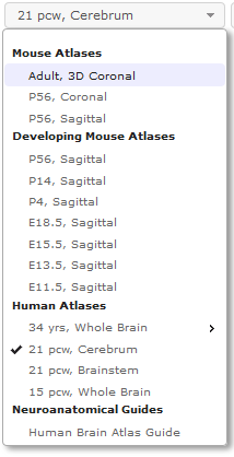
Alternative Background Images
From this menu, you can overlay the annotations over the Nissl image series used to draw the structure polygons.
Settings
The Settings menu allow you to change the settings of the image viewer. From this menu you can download individual images and toggle features such the Atlas or structure metadata, thumbnail image viewing or the various annotations.
Zoom And Pan (ZAP) Image Viewer
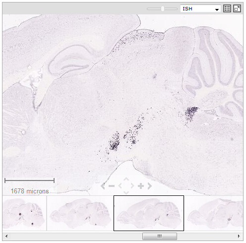
The Zoom and Pan (ZAP) Image Viewer is a powerful tool to navigate and view the images in an experiment. The main part of the viewer is an interactive window where an image can be repositioned by dragging with a mouse. Use the scroll wheel or the keyboard to zoom in or out.
Scale Bar
Drag the scale bar with your mouse to the desired location. Click the text with your mouse to toggle between horizontal and vertical.
Keyboard Commands
Use the keyboard to navigate through the image series. Keyboard commands include:
You can also use the arrow keys to pan the current image.
Using The High Resolution Image Viewer
The Interactive Atlas Viewer has been incorporated into the High Resolution Image Viewer, which is used to look at experimental ISH images in higher resolution.
When viewing an ISH image series either in a gene detail page view or in an experimental image viewer, you can open a High Resolution Image Viewer by clicking on the icon (see below).

Interacting with the High Resolution Image Viewer is similar to using the ZAP Viewer with some enhanced features accessible from icons in the top right hand of the main image viewer.
| Icon | Description |
|---|---|
 | View ISH, Expression Energy, or Reference Stain (Nissl or Feulgen-HP Yellow) |
 | View experiment side by side with the Interactive Reference Atlas |
 | Allows you to access setting options, including downloading the current image |
Side-By-Side Reference Atlas Viewing
To open up the reference atlas in a side-by-side view, click the key icon (see below).

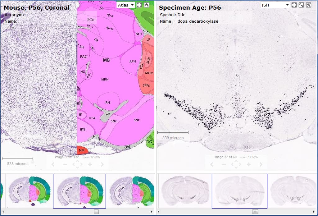
In this view, other options become available at the top of the image viewers
| Icon | Description |
|---|---|
 | Choose between the drawn images or the Nissl stains in the background |
 | Syncs the other image to the current windows section, zoom and pan |
 | Opens the Ontology Hierarchy |
Clicking the Ontology Hierarchy button will open the Ontology in the Atlas window.

Learn about Allen Human Brain Reference Atlas with comprehensive guides and examples from Allen Institute for Brain Science.
Reference Atlases
These anatomical reference atlases illustrate the adult human brain, using modified Brodmann or gyral annotation. The Neuroanatomic Reference Guide is meant to provide a spatial context for the anatomic structures of the Adult Human Brain.
Modified Brodmann
The 2D coronal reference atlas is annotated on Nissl sections from a 34-year-old female based on a modified Brodmann nomenclature. It provides spatial context for gene expression in the Allen Human Brain Atlas and the BrainSpan Atlas of the Developing Human Brain.
106 coronal sections at 0.4 - 3.4 mm intervals
Gyral
The 2D coronal reference atlas is annotated on Nissl sections from a 34-year-old female, by gyrus. It provides spatial context for gene expression in the Allen Human Brain Atlas and the BrainSpan Atlas of the Developing Human Brain.
106 coronal sections at 0.4 - 3.4 mm intervals
Neuroanatomic Reference Guide

From the heatmap view in the Human Brain Atlas, you can see the Structure Ontology list from the selected data point in the heatmap. Clicking on the link at the bottom of the structure ontology list above the heatmap in the Human Brain Atlas will bring you to the Human Brain Atlas Guide.
From the In Situ Hybridization data in the Human Brain Atlas, you can also arrive at the Human Brain Atlas Guide by clicking on a hotspot while viewing an experiment in the High Resolution Image Viewer.
Either of these actions will bring you to the Interactive Atlas Viewer with the structure of interest highlighted in purple.
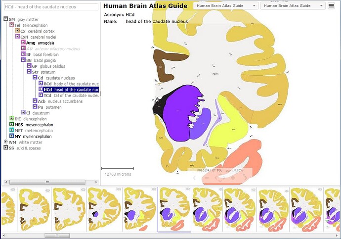
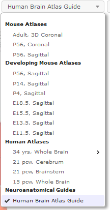
You can also reach this guide by selecting “Human Brain Atlas Guide” from the first drop-down menu in the top right-hand corner whilst in any of the reference atlases in the Interactive Atlas Viewer.
Reference Atlas Viewing Tools
Interactive Atlas Viewer (IAV)
Zoom-And-Pan (ZAP) Image Viewer
Using The High Resolution Image Viewer
Learn about Allen Developing Mouse Brain Reference Atlas with comprehensive guides and examples from Allen Institute for Brain Science.
Reference Datasets
To provide a neuroanatomical framework for gene expression data, the Allen Developing Mouse Brain Reference Atlas was created with the expertise of Professor Luis Puelles, M.D., Ph.D. (University of Murcia, Spain). Sagittal full-color, high resolution web-based digital reference atlases have been created for seven stages of mouse brain development accompanied by a systematic developmental taxonomy of mouse brain structures.
The Allen Developing Mouse Brain Reference Atlases were designed to:
- Allow users to directly compare gene expression patterns to an annotated developmental atlas;
- Provide templates for the creation of 3-D computer models of the developing mouse brain;
- Serve as a neuroanatomical foundation for informatics-based analysis tools.
In 2013, the reference atlas was updated to provide a deeper level of annotation. For more information on the reference atlas update and a description of the ontological levels, please refer to the Reference Atlas whitepaper located under the Documentation tab. Access to the previous reference datasets are available via links on the Reference Atlas landing page.
To access the reference atlas, you can click on one of the links from the landing page or you can select the key icon from the High Resolution Image Viewer to view the atlas in context with a gene expression experiment.
From the Reference Atlas landing page, you can also add reference data into your cart to enhance your exploration of gene expression data by clicking the checkboxes next to the desired reference dataset. Clicking “View Experiments” will allow you to view all selected datasets (including experimental data already present in the cart).
Translation Between the Adult and Developing Mouse Ontologies
Given there are two structure ontologies for the mouse brain in the Allen Brain Atlas resources, we have created a way to overlay the Structure Ontology from Adult Mouse Atlas and the Developing Mouse Brain Atlas.
While in the “Developing Mouse Atlas, P56”, select “P56 Adult Mouse” atlas from the second drop-down menu and select “Outlines” from the Tools icon drop-down. This will show both Structure Ontologies overlayed together.
Reference Atlas Viewing with Gene Expression Data
Structure Ontology
The Structure Ontology for the Developing Mouse is listed hierarchically in the left-hand panel of the Interactive Atlas Viewer. By default the atlas is opened to level 3. Please see the Reference Atlas whitepaper available from the Documentation tab for more information on the Structure Ontology levels.
Each of the Developing Mouse atlases was drawn to a specific level and only those levels that were drawn will be available to navigate by clicking on the name. Those that are not available will be greyed out. Clicking on a structure name will take you to that drawn structure in the main image viewer.
Ontology Levels
Clicking on the ontology icon (see below) will open up the Developing Mouse Ontology defaulting at level 3.
The ontology levels in the Developing Mouse Atlas range from Level 00 (Neural Plate) up through higher differentiation levels to Level 13. Please see the Reference Atlas whitepaper available from the Documentation tab for a deeper explanation of the ontology levels. By clicking on the Ontology Levels (numbered squares above the ontology list) you will open the ontology to the level of detail indicated by the highlighted level.
Searching using the text box in the Ontology pane will allow you to browse through the ontology looking for specific regions. Using the “Sync” icon (see below), you can sync either image to its partner to view the gene expression in context with the reference atlas.
Given the difficulty of sectioning and programatically aligning these small specimen, you have the option of viewing a reference dataset with each gene expression specimen that will also outline a small structure of interest. To do this, choose the reference atlas from the Atlas dropdown menu (either Feulgen-HP or Nissl, depending upon the age) and select on the reference data set to outline your desired structure.
In the below image, gene expression is located in a region of the prethalamus.
Reference Atlas Viewing Tools
Interactive Atlas Viewer (IAV)
Zoom-And-Pan (ZAP) Image Viewer
Using The High Resolution Image Viewer
Learn about Brainspan Atlas Of The Developing Human with comprehensive guides and examples from Allen Institute for Brain Science.
Reference Atlases
To complement the RNA-Seq and microarray gene expression data, reference atlases were created at three developmental stages; 15 pcw, 21 pcw and 34 years. The reference atlas are full-color, high-resolution, web-based digital brain atlases accompanied by a systematic, hierarchically organized taxonomy of developing brain structures.
From the heatmap view in the BrainSpan Atlas of the Developing Human Brain, you can see the Structure Ontology list from the selected data point in the heatmap. Clicking on the structure link will bring you to the appropriate developmental stage in the Reference Atlas (adult vs. prenatal).
From the In Situ Hybridization data in the BrainSpan Atlas of the Developing Human Brain, you can also arrive at the Human Brain Atlas Guide by clicking on a hotspot while viewing an experiment in the High Resolution Image Viewer.
Either of these actions will bring you to the Interactive Atlas Viewer with the structure of interest highlighted in purple.
Clicking on the annotation links from the “Reference Atlas” tab in the banner menu will also take you to the Interactive Atlas Viewers. Supporting data used to create these Atlases is also available for viewing or for download.
Reference Atlas Viewing Tools
Interactive Atlas Viewer (IAV)
Zoom-And-Pan (ZAP) Image Viewer
Using The High Resolution Image Viewer
Learn about Mouse Spinal Cord Reference Atlases with comprehensive guides and examples from Allen Institute for Brain Science.
Reference Atlases
These anatomical reference atlases illustrate the mouse spinal cord in adult and juvenile C57BL/6J mouse. They provide a spatial map for the Allen Mouse Spinal Cord Atlases of gene expression. Dr. Charles Watson and Dr, Gulgun Kayalioglu created a custom taxonomy for annotation of the spinal cord, covering cervical, thoracic, lumbar, sacral, and coccygeal segments.
Age P4
The 2D sagittal reference atlas is annotated on Nissl sections collected from a juvenile male C57BL/6J mouse, postnatal day 4 (P4). It provides the spatial context for in situ hybridization-based gene expression in Allen Mouse Spinal Cord Atlas.
34 transverse sections at 2 mm intervals
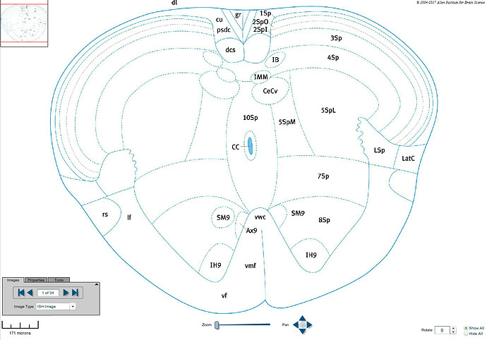
Age P56
The 2D sagittal reference atlas is annotated on Nissl sections collected from an adult male C57BL/6J mouse, postnatal day 56 (P56). It provides the spatial context for in situ hybridization-based gene expression in Allen Mouse Spinal Cord Atlas.
34 transverse sections at 2 mm intervals
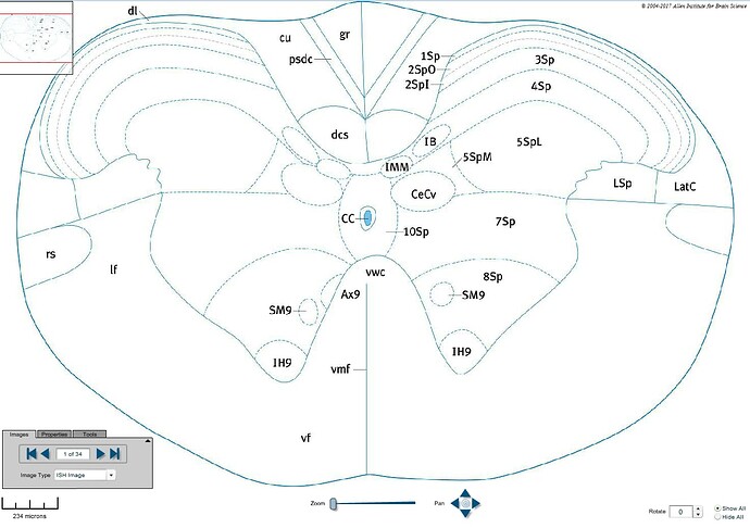
Reference Atlas Viewing Tools
Interactive Atlas Viewer (IAV)
Zoom-And-Pan (ZAP) Image Viewer
Using The High Resolution Image Viewer
Learn about Adult Mouse Brain Reference Atlas with comprehensive guides and examples from Allen Institute for Brain Science.
Reference Atlases
The Allen Reference Atlases are designed to:
- Allow users to directly compare data to neuroanatomical structures.
- Serve as templates for the development of 3-D computer graphic models of mouse brain, providing a foundation for the development of informatics-based annotation tools.
- Provide a standard neuroanatomical ontology for determining structural annotation and aid in the construction of a detailed searchable gene expression database.
Adult, 3-D Coronal
This coronal reference atlas is created from a 3-D volumetric reference atlas, annotated symmetrically using an average of data merged from 1,675 brain specimens. It provides spatial context and a common coordinate framework for mapping data in the Allen Mouse Connectivity Atlas, the Allen Cell Types Database (mouse), and the Allen Brain Observatory. This 2-D atlas consists of 132 virtual planes at 100 µm intervals.
P56, 2-D Atlases
These mouse reference atlases were created by Hong Wei Dong, M.D., Ph.D., in the coronal and the sagittal plane. They are full-color, high-resolution, web-based digital brain atlases accompanied by a systematic, hierarchically organized taxonomy of mouse brain structures. The gene expression data and reference atlases are derived using identical methodology, from 8-week old C57BL/6J male mouse brains prepared as unfixed, fresh-frozen tissue.
The coronal reference atlas consists of 132 coronal sections evenly spaced at 100 µm intervals and annotated to a detail of numerous brain structures. The sagittal reference atlas consists of 21 representative sagittal sections spaced at 200 µm intervals, annotated for 71 major brain regions.
The Allen Reference Atlas was first released online in 2005, and underwent several updates to add increasing complexity to the neuroanatomic delineations. Version 1 (2008) is used on the website to refer to the version of the atlas that was completed for publication as the print atlas (Dong, 2008) and used as the primary reference atlas in the Allen Mouse Brain Atlas until November 2011. Version 2 (2011) was developed to enable interactive exploration of the atlas online.
From the Reference Atlas landing page in the Allen Mouse Brain Atlas, you can explore the atlases in the Interactive Atlas Viewer or you can view the static 2008 versions of the images.
Reference Atlas Viewing Tools
Interactive Atlas Viewer (IAV)
Zoom-And-Pan (ZAP) Image Viewer
Using The High Resolution Image Viewer

Learn about Rna Seq Process Controls with comprehensive guides and examples from Allen Institute for Brain Science.
To monitor for consistent, high-quality sampling of single-cell and single-nucleus RNA-Seq data, eight controls (4 negative and 4 positive) were included in each Amplification set (8 controls + 88 samples). A control strip included 2 wells without cells (termed ERCC for External RNA Controls Consortium, negative), 2 wells without cells or ERCC (termed NTC for No Template Control, negative), 2 wells with 10 pg Control RNA (mouse) provided in the Takara SMART-Seq v4 kit (termed Control RNA, positive), and 2 wells with either 10 pg of Mouse Whole Brain Total RNA (termed MouseWhole, Zyagen MR-201, positive) or 10 pg of Human Universal Reference Total RNA (termed UHR, Takara 636538, positive). Controls for mouse and human data is available to download via the links below, and detailed methods are described in the Technical Whitepapers.
Note that separate control sets are available for samples released in June 2018 and October 2018.
Download
Human MTG: Controls Data | .gtf File
Human VISp and ACC: Controls Data | .gtf File
Mouse VISp & ALM: Controls Data | .gtf File
Mouse ACA & MOp (cells and nuclei): Controls Data | .gtf File
Learn about Human Multiple Cortical Areas with comprehensive guides and examples from Allen Institute for Brain Science.
Overview and Experimental Strategy
To investigate the cellular diversity across human cortex, a low-bias approach to profile cell-type diversity was sought, constrained by the challenge of working with precious and limited tissue sources. Individual layers of cortex were dissected from tissues covering the middle temporal gyrus (MTG), anterior cingulate gyrus (CgGr), primary visual cortex (V1C), primary motor cortex (M1C), primary somatosensory cortex (S1C) and primary auditory cortex (A1C) derived from human brain, and nuclei were dissociated and sorted using the neuronal marker NeuN. Nuclei were sampled from postmortem and neurosurgical (MTG only) donor brains, and expression was profiled with SMART-Seq v4 or 10x v3 RNA-sequencing.
Human Tissue: Case Qualification
This database of cell types includes experimental data derived from adult human brain. Human brain tissue samples from either postmortem or neurosurgical origin were made available through the generosity of tissue donors. Clinical summaries and donor characteristics are provided in this document as well as a description of the criteria for acceptance of use in this study.
Tissue Preparation and Single Nucleus Dissociation and Sorting
To prepare and archive tissues from suitable cases, whole postmortem brain specimens were bisected through the midline, and individual hemispheres were embedded in alginate for slabbing. Coronal brain slabs were cut at 0.5-1cm intervals through each hemisphere and the slabs were then frozen in a bath of dry ice and isopentane, vacuum sealed in freezer bags to prevent frost damage, and stored at -80°C until use. Regions of interest were subsequently removed from tissue slabs, sectioned on a vibratome and processed for nuclei isolation.
Neurosurgical donor tissue (MTG only) was received from patients undergoing surgery for epilepsy or brain tumors. The tissue blocks received were distal, apparently normal cortical tissue removed to access underlying pathological brain tissues. Tissue was transported in chilled ACSF, sectioned at 350µm and stored at -80°C until they were processed for nuclei isolation.
Single nuclei were captured by gating on DAPI-positive events, excluding debris and doublets, and then gating on NeuN signal, which allowed for the isolation of either NeuN-positive (neuronal) or NeuN-negative (non-neuronal) events.
PROTOCOL Human Tissue Sectioning and Dissection for Nuclear Isolation
PROTOCOL Isolation of Nuclei from Adult Human Brain Tissue
PROTOCOL Isolation of Nuclei from Adult Brain Tissue from 10x Genomics Platform
SMART-seq v4 RNA-Sequencing
SMART-Seq v4 Ultra Low Input RNA Kit for Sequencing (Takara #634894) was used per the manufacturer’s instructions for cDNA synthesis of single-cell RNA and subsequent amplification. Sequencing libraries were prepared using the NexteraXT DNA Library Preparation kit (Illumina FC-131-1096) with NexteraXT Index Kit V2 Set A, B, C, or D (FC-131-2001, 2002, 2003, or 2004) or custom 8-base or 10-base Unique Design index primers designed and manufactured by IDT (Integrated DNA Technologies). NexteraXT DNA Library prep was done at either 0.5x volume manually or 0.4x or 0.2x volume on the Mantis instrument (Formulatrix). Pooled sequencing libraries were sent to an outside vendor for sequencing on an Illumina HiSeq 2500 instrument. All of the library pools were run using Illumina High Output V4 chemistry. RNA sequencing services were provided by Covance Genomics Laboratory, Seattle subsidiary of LabCorp Group of Holdings, and The Broad Institute Genome Sequencing Platform.
PROTOCOL Nextera XT at 0.2X on the Mantis
PROTOCOL SMART-Seq v4 (1x) amplification
PROTOCOL SMART-Seq v4 (0.5x) amplification
SMART-seq v4 Gene Expression Quantification
Raw read (fastq) files were aligned to the GRCh28 human genome sequence (Genome Reference Consortium, 2011) with the RefSeq transcriptome version GRCh28.p2 (current as of 4/13/2015) and updated by removing duplicate Entrez gene entries from the gtf reference file for STAR processing. For alignment, Illumina sequencing adapters were clipped from the reads using the fastqMCF program. After clipping, the paired-end reads were mapped using Spliced Transcripts Alignment to a Reference (STAR) using default settings. Reads that did not map to the genome were then aligned to synthetic construct (i.e. ERCC) sequences and the E. coli genome (version ASM584v2). Quantification was performed using summerizeOverlaps from the R package GenomicAlignments. Expression levels were calculated as counts per million (CPM) of exonic plus intronic reads.
10x Chromium RNA-sequencing
Single nucleus suspensions were frozen in a solution of 1X PBS, 1% BSA, 10% DMSO, and 0.5% RNAsin Plus RNase inhibitor (Promega, N2611) and stored at -80°C. At the time of use, frozen nuclei were thawed at 37°C and processed for loading on the 10x Chromium instrument as described (dx.doi.org/10.17504/protocols.io.nx3dfqn). Samples were processed using the 10x Chromium Single Cell 3’ Reagent Kit v3. 10x chip loading and sample processing was done according to the manufacturer’s protocol. Gene expression was quantified using the default 10x Cell Ranger v3 pipeline except substituting the curated genome annotation used for SMART-seq v4 quantification. Introns were annotated as “mRNA,” and intronic reads were included in expression quantification.
Cell Type Clustering
Nuclei were included in the clustering analysis if they passed all QC criteria.
SMART-seq v4 criteria:
- > 30% cDNA longer than 400 base pairs
- > 500,000 reads aligned to exonic or intronic sequence
- > 40% of total reads aligned
- > 50% unique reads
- > 0.7 TA nucleotide ratio
10x v3 criteria:
- > 500 (non-neuronal cells) or > 1000 (neuronal cells) genes detected
- < 0.3 doublet score
Nuclei passing QC criteria were grouped into transcriptomic cell types using an iterative clustering procedure previously reported in (Tasic et al. 2018; Hodge, Bakken et al., 2019). Briefly, intronic and exonic read counts were summed, and log2-transformed expression was centered and scaled across nuclei. X- and Y-chromosomes and mitochondrial genes were excluded to avoid nuclei clustering based on sex or nuclei quality. Differentially expressed genes were selected, principal components analysis (PCA) reduced dimensionality, and a nearest neighbor graph was built using up to 20 principal components. Clusters were identified with Louvain community detection (or Ward's hierarchical clustering if N < 3000 nuclei), and pairs of clusters were merged if either cluster lacked marker genes. Clustering was applied iteratively to each sub-cluster until clusters could not be further split.
Cluster robustness was assessed by repeating iterative clustering 100 times for random subsets of 80% of nuclei. A co-clustering matrix was generated that represented the proportion of clustering iterations that each pair of nuclei were assigned to the same cluster. We defined consensus clusters by iteratively splitting the co-clustering matrix as described (Tasic et al. 2018; Hodge, Bakken et al., 2019).
Clusters were curated based on outlier values of the initial QC values or cell class marker expression (GAD1, SLC17A7, SNAP25). Clusters were identified as donor-specific if they included fewer nuclei sampled from donors than expected by chance. To confirm exclusion, clusters automatically flagged as outliers or donor-specific were manually inspected for expression of broad cell class marker genes, mitochondrial genes related to quality, and known activity-dependent genes.
The clustering pipeline is implemented in the R package “scrattch.hicat”, and the clustering method is provided by the “run_consensus_clust” function.
CODE Hierarchical, iterative clustering for analysis of transcriptomics data in R
Funding
Data generation was supported by multiple awards, including Brain Initiative Cell Census Network (BICCN) award U01MH114812 from the National Institute of Mental Health and the National Institute of Neurological Disorders and Stroke, and by the Allen Institute for Brain Science.
References
Hodge, R.D., Bakken, T.E., et al. (2019). "Conserved cell types with divergent features in human versus mouse cortex." Nature 573:61-68. PMID DOI
Tasic, B., et al. (2018). "Shared and distinct transcriptomic cell types across neocortical areas." Nature 563(7729): 72-78. doi: 10.1038/s41586-018-0654-5. Epub 2018 Oct 31. PMID PMCID DOI
Learn about Mouse Whole Cortex And Hippocampus with comprehensive guides and examples from Allen Institute for Brain Science.
Overview and Experimental Design
Our goal is to quantify the diversity of cell types in the adult mouse brain using large-scale single-cell transcriptomics. Towards that goal, we have generated a dataset that includes single cells from multiple cortical areas and the hippocampus. Samples were collected from fine dissections of brain regions from male and female mice. For most brain regions, we isolated labeled cells from pan-GABAergic, pan-glutamatergic, and pan-neuronal transgenic lines. For primary visual cortex (VISp) and anterolateral motor cortex (ALM), we sampled additional cells using driver lines that label more specific and rare types. To investigate the correspondence between transcriptomic types and neuronal projection properties, we collected cells labeled from retrograde injections for select combinations of target injection sites and dissection regions. Labeled cells were collected by fluorescence activated sorting (FACS) of single cells. We also collected cells without fluorescent labeling to sample non-neuronal cell types. Isolated single cells were processed for RNA sequencing using SMART-Seq v4 and 10x chromium v2. This dataset reveals the molecular architecture of the neocortex and hippocampal formation, with a wide range of shared and unique cell types across areas. It provides the basis for comparative studies of cellular diversity in development, evolution, and diseases.
Tissue Donors and Treatments
Tissue samples were obtained from adult (postnatal day P53-P59) mice, both male and female, carrying one or two recombinase transgenes (Cre, FlpO) and a recombinase-dependent reporter transgene. Detailed descriptions of recombinase and reporter lines can be found in Transgenic Characterization. In addition, retrogradely labeled cells were isolated from reporter mice infected with a Cre-dependent virus, or from wild-type mice infected with a reporter virus.
We injected AAV2-retro-EF1a-Cre (Tervo et al., 2016), RV∆GL-Cre (Chatterjee et al., 2018), or CAV-Cre (gift of Miguel Chillon Rodrigues, Universitat Autònoma de Barcelona) (Hnasko et al., 2006) into brains of heterozygous or homozygous Ai14 mice using established procedures (Tasic et al., 2016, 2018). For ALM experiments, we also injected AAV2-retro-CAG-GFP or AAV2-retro-CAG-tdTomato (Tervo et al., 2016) into wild-type mice. Mice were anesthetized with 5% isoflurane and then placed into a stereotaxic alignment instrument (Kopf, model 1900). Anesthesia was maintained for the duration of the surgery by administering isoflurane at 1-2% through a nose cone. The skin along the midline of the skull was opened using a scalpel, and a surgical drill was used to create a small hole in the skull. A pulled glass pipette prefilled with virus solution was lowered into the brain, and 165-500 nl of the virus solution was delivered to the targeted brain area using a pressure injection system (NanoJect II, Drummond Scientific Company, Catalog# 3-000-204). Stereotaxic coordinates were obtained from Paxinos adult mouse brain atlas (Paxinos and Franklin, 2008). For two VISp experiments, we injected into SCs by inserting the needle through the cerebellum at a 45° angle in the posterior to anterior direction. After the delivery of virus solution into the brain, the glass pipette was retracted and the incision in the scalp was closed using sutures. The animal was removed from the stereotaxic frame and allowed to recover from anesthesia. Mice were sacrificed 7−21 days after surgery for single cell isolation. TdT+ or GFP+ single cells were isolated from cortical areas as described below.
Tissue Preparation and Single Cell Dissociation - Mouse Protocol
Mice were anesthetized with 5% isoflurane and intracardially perfused with ice-cold, oxygenated artificial cerebral spinal fluid (ACSF). The brain was then rapidly dissected and mounted for coronal slice preparation on the chuck of a Compresstome VF-300 vibrating microtome (Precisionary Instruments). Using a custom photodocumentation system (Mako G125B PoE camera with custom integrated software), a blockface image of the coronal or semi-coronal brain surface was acquired before each section was sliced at 250 μm intervals. The slice was then hemisected along the midline, and typically both hemispheres for cortical samples were transferred to ACSF.
Each slice-hemisphere was transferred into a Sylgard-coated dissection dish containing chilled, oxygenated ACSF. Brightfield and fluorescent images between 1X and 20X were obtained of the intact tissue with a Nikon Digital Sight DS-Fi1 or a Sentech STC-SC500POE camera mounted to a Nikon SMZ1500 dissecting microscope. To guide anatomical targeting for dissection, boundaries were identified by trained anatomists, comparing the blockface image and the slice image to a matched plane of the Allen Reference Atlas. In general, three to five slices were sufficient to capture the targeted region of interest, allowing for expression analysis along the anterior-posterior axis. The region of interest was then dissected and both brightfield and fluorescent images of the dissections were acquired for secondary verification. The dissected regions were transferred in ACSF to a microcentrifuge tube and stored on ice. This process was repeated for all slices containing the target region of interest, with each region of interest deposited into a new microcentrifuge tube.
After all regions of interest were dissected, the tissue pieces were digested in an ACSF solution containing 2 mg/ml of pronase (before 6/21/2018) or 30 U/ml of papain (after 6/21/2018). With pronase, the tissue was incubated at room temperature (approximately 22°C) for a duration that consisted of adding 15 minutes to the age of the mouse (in days; i.e., P53 specimen had a digestion time of 68 minutes). With papain, the tissue was incubated in a dry oven at 35°C (target solution temperature of 30°C) for 30 minutes. After digestion, the enzymatic solution was removed and a quenching buffer (1% FBS or 1% BSA) was added. The tissue was washed two more times with the quenching solution with the third wash being 500 μl for final sample volume. The sample was then triturated using fire-polished glass pipettes of decreasing bore sizes (600, 350 and 150 μm). The cell suspension was incubated on ice in preparation for fluorescence-activated cell sorting (FACS).
Note: Samples collected after 12/16/2016 had 0.0132M trehalose added to all solutions used after the point of slicing to improve cell viability and yield.
PROTOCOL Slice Preparation with Tissue Dissociation - Mouse Protocol
Single Cell Sorting
Samples were prepared for sorting by passing the suspension through a 70-µm filter and adding DAPI (to the final concentration of 2 ng/ml).
Single cells were sorted by excluding DAPI positive events and debris, and gating to include red fluorescent events (tdTomato-positive cells) or green fluorescent events (GFP-positive cells).
For SmartSeq v4, single cells were sorted into individual wells of 8-well PCR strips containing lysis buffer from the SMART-Seq v4 kit with RNase inhibitor (0.17 U/μl), immediately frozen on dry ice, and stored at −80 °C. For 10x Genomics, 30,000 cells were sorted within 10 minutes into a tube containing 500 µl of quenching buffer. Each aliquot of 30,000 sorted cells was layered on top of a high concentration BSA buffer and immediately centrifuged at 230xg for 10 minutes in a swinging bucket centrifuge. Supernatant was removed and 35 µl of buffer was left behind, in which the cell pellet was resuspended. The cell concentration was quantified and loaded onto the 10x Genomics Chromium controller.
PROTOCOL FACS Single Cell Sorting V.2
RNA Sequencing
For SMART-Seq v4 processing, the SMART-Seq v4 Ultra Low Input RNA Kit for Sequencing (Takara #634894) was used per the manufacturer’s instructions for cDNA synthesis of single-cell RNA and subsequent amplification. Sequencing libraries were prepared using the NexteraXT DNA Library Preparation kit (Illumina FC-131-1096) with NexteraXT Index Kit V2 Set A, B, C, or D (FC-131-2001, 2002, 2003, or 2004) or custom 8-base or 10-base Unique Design index primers designed and manufactured by IDT (Integrated DNA Technologies). NexteraXT DNA Library prep was done at either 0.5x volume manually or 0.4x or 0.2x volume on the Mantis instrument (Formulatrix). Pooled sequencing libraries were sent to an outside vendor for sequencing on an Illumina HiSeq 2500 instrument. All the library pools were run using Illumina High Output V4 chemistry. RNA sequencing services were provided by Covance Genomics Laboratory, Seattle subsidiary of LabCorp Group of Holdings, and The Broad Institute Genome Sequencing Platform.
For 10xv2 processing, we used Chromium Single Cell 3’ Reagent Kit v2 (10x Genomics Cat# 120237). We followed manufacturer’s instructions for cell capture, barcoding, reverse transcription, cDNA amplification, and library construction. 10xv2 libraries were sequenced on Illumina NovaSeq6000.
PROTOCOL Nextera XT at 0.2X on the Mantis
PROTOCOL SMART-Seq v4 (1x) amplification
PROTOCOL SMART-Seq v4 (0.5x) amplification
PROTOCOL 10Xv2 RNASeq Sample Processing
RNAseq Gene Expression Quantification and Quality Control
From raw SMART-Seq v4 reads, the Illumina sequencing adapters were clipped using the fastqMCF program. After clipping, the paired-end reads were aligned to the mm10 mouse genome sequence (Genome Reference Consortium, 2011) with the RefSeq transcriptome version GRCm38.p3 (current as of 01/15/2016) and updated by removing duplicate Entrez gene entries from the gtf reference file using Spliced Transcripts Alignment to a Reference (STAR v2.5.3) (Dobin, et al., 2013) with default settings. Reads that did not map to the genome were then aligned to synthetic construct (i.e. ERCC) sequences and the E.coli genome (version ASM584v2). The output files included quantification of the uniquely mapped reads (raw exon and intron counts for the transcriptome-mapped reads). The vast majority of reads could be mapped uniquely to the reference. The output files further contained the percentages of reads mapped to the transcriptome, to ERCC spike-in controls, and to E.coli. These metrics were used for quality control assessments. Quantification of mapped reads was performed using summerizeOverlaps from the R package GenomicAlignments. Expression levels were calculated as counts per million (CPM) of exonic plus intronic reads. Gene detection was calculated as the number of genes expressed in each sample with CPM > 0. Cells were included in downstream analysis if they passed all of the following QC thresholds:
- > 100,000 total reads
- > 75% total reads aligned
- > 1000 genes with CPM
- < 0.5 CG complexity
10xv2 sequencing reads were aligned to the mouse pre-mRNA reference transcriptome (mm10) using the 10x Genomics CellRanger pipeline (version 3.0.0) with default parameters. Cells were classified into broad classes of excitatory, inhibitory, and non-neuronal based on known markers. Cells that met the following criteria were filtered out for downstream processing: neurons with fewer than 2000 detected genes and non-neuronal cells with fewer than 1000 detected genes. Doublets were identified using a modified version of the DoubletFinder algorithm {McGinnes 2019} and removed when doublet score > 0.3.
Analysis and Clustering
Cells were grouped into transcriptomic cell types using the iterative clustering procedure described in Tasic et al. 2018. Predicted gene models (gene names that start with Gm), genes from the mitochondrial chromosome, ribosomal genes and sex-specific genes were removed from downstream analysis. All quality control qualified cells were clustered following the steps of high variance gene selection, dimensionality reduction, dimension filtering, Jaccard–Louvain clustering, and cluster merging. Differential gene expression (DGE) was computed for every pair of clusters, and pairs that did not meet the DGE criteria were merged. Differentially expressed genes were defined using two criteria: 1) significant differential expression (> 2-fold; Benjamini-Hochberg false discovery rate < 0.01) and 2) binary expression (CPM > 1 in more the half of cells in one cluster and < 30% of this proportion in the other cluster). We define the deScore as the sum of the −log10(false discovery rate) of all differentially expressed genes (each gene contributes to no more than 20), and pairs of clusters with deScore < 150 were merged. This process was repeated within each resulting cluster until no more child clusters met DGE or cluster size (min. 4 cells) criteria. The entire clustering procedure was repeated 100 times using 80% of all cells sampled at random, and the frequency with which cells co-cluster was used to generate a final set of clusters, again subject to differential gene expression and cluster size termination criteria.
The clustering pipeline is implemented in an R package publicly available at github. The clustering method is provided by run_consensus_clust function.
Code Hierarchical, iterative clustering for analysis of transcriptomics data in R
Funding
Data generation was supported by multiple awards, including award U01MH105982 from the National Institute of Mental Health and the Eunice Kennedy Shriver National Institute of Child Health & Human Development, Brain Initiative Cell Census Network (BICCN) award U19MH114830 from the National Institute of Neurological Disorders and Stroke and the National Institute of Mental Health, and by the Allen Institute for Brain Science.
References
Chatterjee, S., et al. (2018). "Nontoxic, double-deletion-mutant rabies viral vectors for retrograde targeting of projection neurons." Nat Neurosci 21(4): 638-646. doi: 10.1038/s41593-018-0091-7. Epub 2018 Mar 5. PMID PMCID DOI
Hnasko, T. S., et al. (2006). "Cre recombinase-mediated restoration of nigrostriatal dopamine in dopamine-deficient mice reverses hypophagia and bradykinesia." Proc Natl Acad Sci U S A 103(23): 8858-8863. doi: 10.1073/pnas.0603081103. Epub 2006 May 24. PMID PMCID DOI
Paxinos, G. and K. B. J. Franklin (2008). "Mouse brain in stereotaxic coordinates 3rd edition." (Academic Press, Cambridge, MA, 2008).
Tasic, B., et al. (2016). "Adult mouse cortical cell taxonomy revealed by single cell transcriptomics." Nat Neurosci 19(2): 335-346. doi: 10.1038/nn.4216. Epub 2016 Jan 4. PMID PMCID DOI
Tasic, B., et al. (2018). "Shared and distinct transcriptomic cell types across neocortical areas." Nature 563(7729): 72-78. doi: 10.1038/s41586-018-0654-5. Epub 2018 Oct 31. PMID PMCID DOI
Tervo, D. G., et al. (2016). "A Designer AAV Variant Permits Efficient Retrograde Access to Projection Neurons." Neuron 92(2): 372-382. doi: 10.1016/j.neuron.2016.09.021. Epub 2016 Oct 6. PMID PMCID DOI
Learn about Synaptic Physiology Analysis Methods Quality Control with comprehensive guides and examples from Allen Institute for Brain Science.
Ensuring the quality of the Synaptic Physiology Dataset is of critical importance. We applied quality control criteria at several stages of data processing and analysis. During the processing stages, in order for data to proceed into successive stages it had to pass quality control for the prior stage. During analysis of connection properties, each analysis (e.g., strength, kinetics, short-term plasticity) had independent quality control metrics. Below is a workflow of the quality control metrics required for inclusion at each stage of processing and analysis.
Data Processing
Data was first processed to ensure that it was of good enough quality to detect a connection
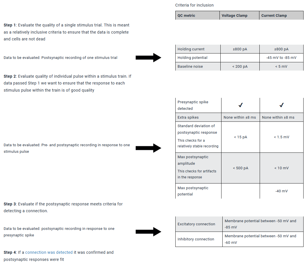
Data analysis
During characterization of a synapse, different QC criteria were applied based on the metric that was being analyzed.
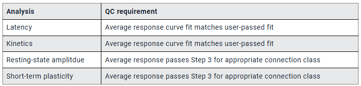
Learn about Synaptic Physiology Analysis Methods Connection Characterization with comprehensive guides and examples from Allen Institute for Brain Science.
Chemical connections were detected manually, curve fit, and then characterized for strength, kinetics, and short-term plasticity in a multi-stage process. Manual connectivity calls were used to train a machine classifier (see Seeman, Campagnola, et al. 2018 for more detail). After training, the machine classifier revealed a set of potential false positives or false negatives that were manually re-checked. Electrical connections were also detected and characterized.
Connection Detection
Chemical connections were visually identified from average postsynaptic responses sorted by recording mode (voltage and current clamp) and membrane potential (see QC criteria for holding potential ranges for excitatory and inhibitory connections). Individual responses were time aligned to the presynaptic spike. Responses that failed QC were not included in the average.
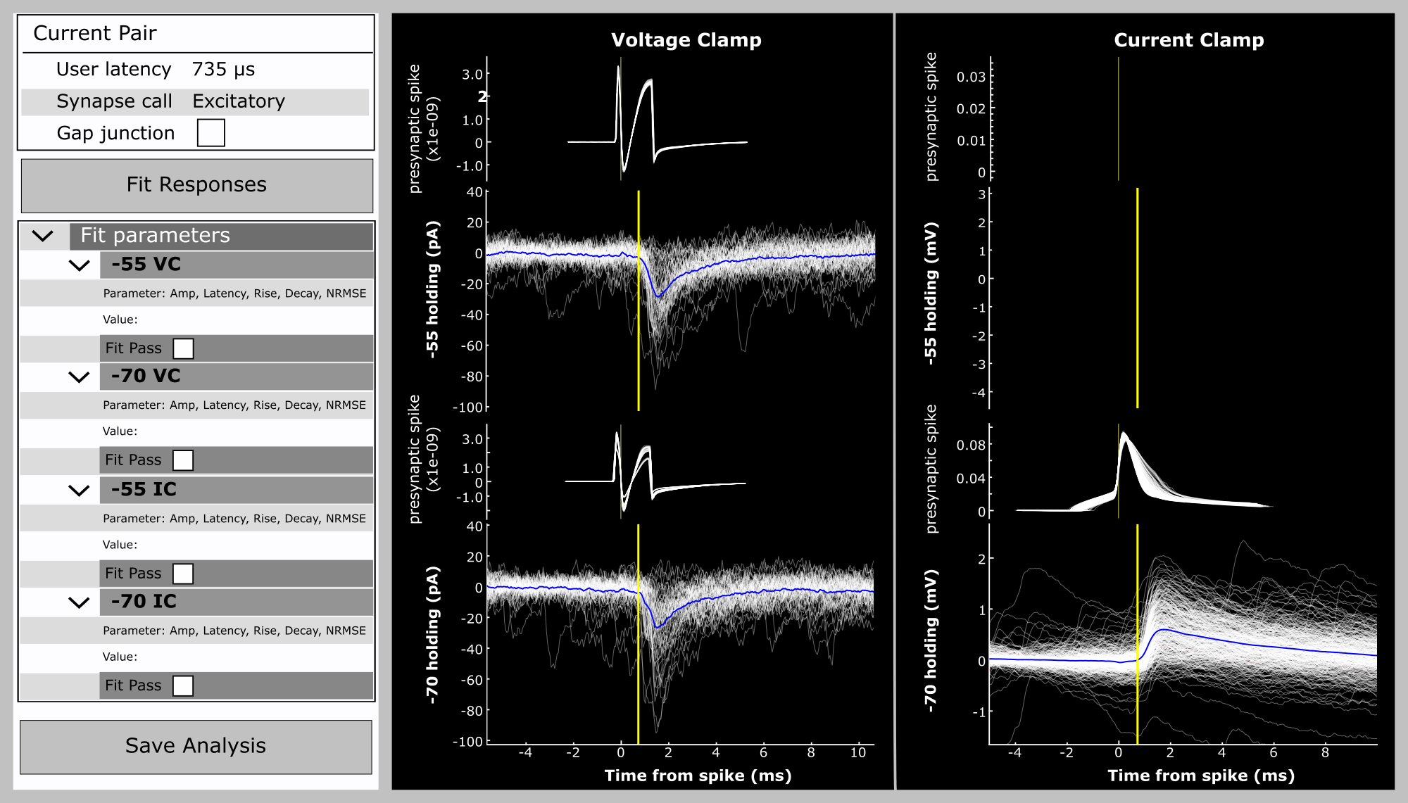
The User Latency value was used to initialize automated curve fitting of the postsynaptic response. Parameters from the curve fits were shown for each quadrant. When the user was satisfied with the curve fitting output, the goodness of fit was manually passed or failed. The user would take into consideration gap junctions, electrical artifacts, the shape of the fit or other factors when deciding whether the curve fit accurately reflected the response. Notes were also made by the user and used to update, and subsequently test, new fitting algorithms.
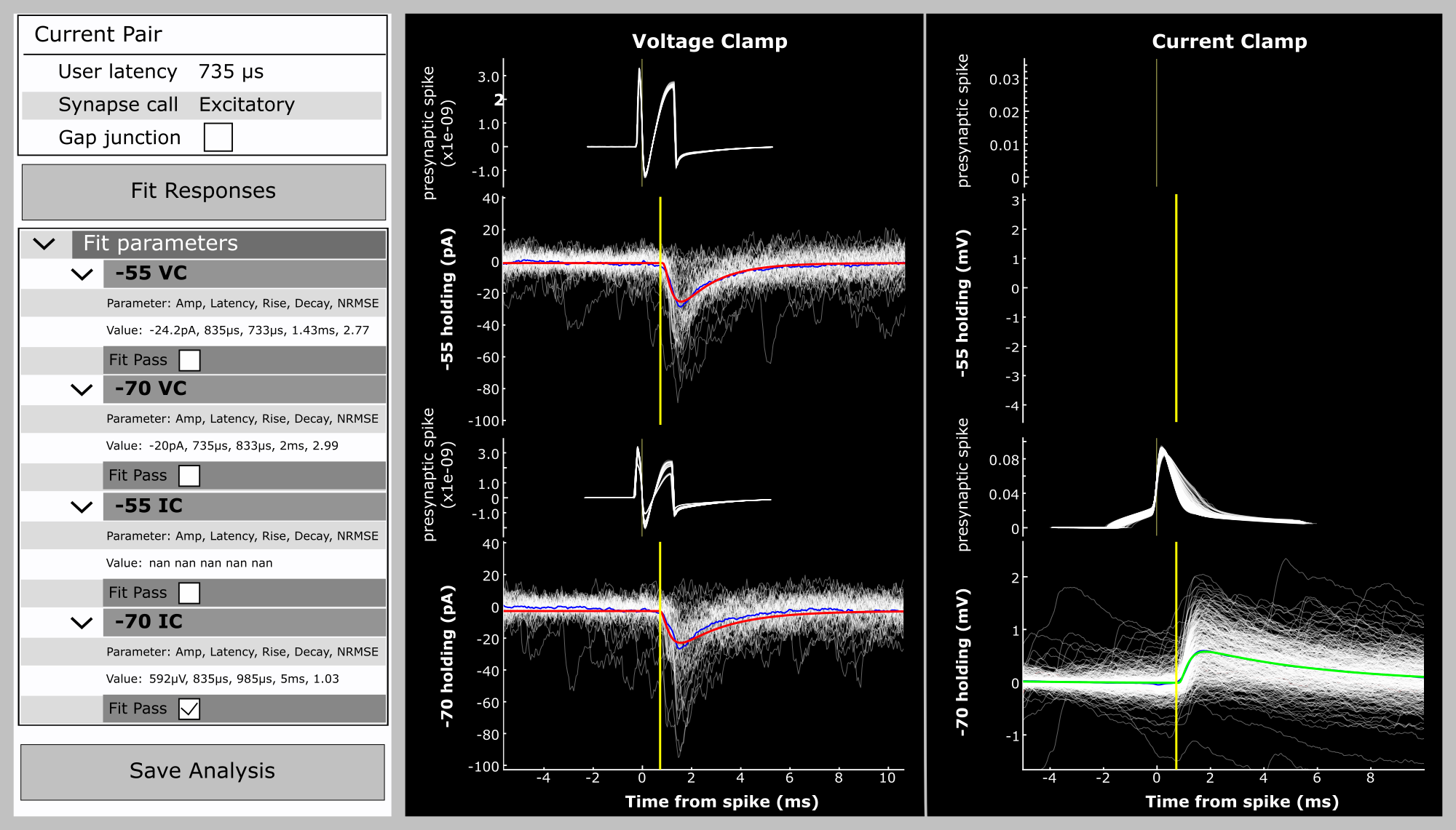
Connection Characterization
Once a chemical connection was identified, the strength and kinetics of that connection, as well as the dynamics (short-term plasticity (STP) and variability), were characterized utilizing the curve fits generated during connection detection.
Strength and Kinetics
The "strength" of a connection is an important characteristic particularly when we want to start comparing connections across cell class. However, we know that strength changes dynamically over time (as is highlighted in our analysis of STP) as well as stochastically from spike to spike. Given that our stimulus set utilizes trains of various frequencies we want to ensure that our metric of strength would be useful in comparisons across connections and not be stimulus dependent. Our resting-state strength is a metric that works well for most connections; however, some facilitating connections have a very small resting-state strength which may be misleading. Rise and decay kinetics are more faithfully preserved even as the amplitude of the connection changes and thus, was more straightforward to characterize.
Resting-state amplitude was determined from responses in which the presynaptic spike follows a period of quiescence. Usually this is the first pulse in each stimulus train. Individual responses were averaged and curve fit; the amplitude output of the fit served as our metric of strength.
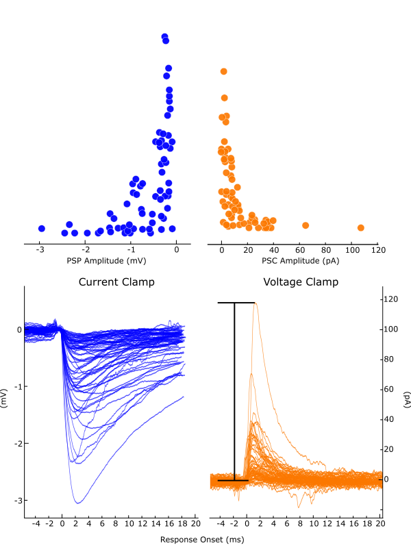
Latency, rise and decay kinetics were also determined from curve fits to average synaptic responses. Kinetics were calculated for postsynaptic currents (PSCs) and potentials (PSPs) held at either -70 or -55 mV depending on whether the synapse was excitatory or inhibitory (see QC requirement).
Short-term plasticity
Short-term plasticity was analyzed from data recorded in current clamp utilizing different stimuli depending on the analysis. We measured three main metrics of short-term plasticity: paired-pulse ratio (PPR), train-induced STP, and recovery from train-induced STP.
Short-term plasticity is often calculated as a ratio of response amplitudes for each pulse in the stimulus train. Many connections in our dataset have small responses that are close to the noise level in our recordings making the use of an amplitude ratio unstable. This situation is accentuated for connections that are strongly depressing or facilitating resulting in spurious ratio measurements. To avoid this instability, we use the 90th percentile PSP amplitude as an approximation of the "maximum" amplitude of a synapse and normalize our STP measurements by this value. Below are the calculations for each STP metric.
Paired-pulse STP was measured from the 50Hz stimulus as:

Train-induced STP was measured from the 50 Hz stimulus as:

Recovery from STP was measured from all stimulus frequencies with a 250 ms delay between the last induction pulse (8th) and first recovery pulse (9th):

Variability
The amplitude of PSPs for a synaptic connection vary randomly each time neurotransmitter is released. This is often reported using the coefficient of variation (CV). In the mouse cortex, however, typical PSP amplitudes can be much smaller than the background electrical noise in the cell. CV in this regime is thus dominated by noise and tells us little about the physiology of the synaptic connections. In our dataset, PSP amplitude variability is reported using a metric that is adjusted (aCV) to correct for the effect of background noise:

This metric has a value of 1.0 when the standard deviation of the PSP amplitudes (after noise correction) is the same as the median amplitude. The noise correction itself introduces a new source of variance, however, which can sometimes lead to this value being negative. We measure variability in the resting state for each connection as well as in various states of induced short-term plasticity.

Synaptic Vesicle Release Model
We developed a new model of synaptic vesicle release that provides a more comprehensive description of each synaptic connection and also allows to predict the behavior of the synapse in response to arbitrary stimuli. The model includes basic quantal release parameters (release probability, number of release sites, and quantal size) as well as short term plasticity (vesicle depletion, depression, and facilitation with varying recovery time constants) and accounts for recording noise.
Our dataset includes best fit parameters (using a maximum likelihood estimation) of the model for many connections that can be used to simulate different types of connections, or as a basis for comparison between connection types.
Electrical Connections
Electrical connections, formed by gap junctions, were also detected in our dataset. We used the long-pulse stimuli to characterize the strength of electrical connections.
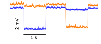
Learn about Synaptic Physiology Analysis Methods with comprehensive guides and examples from Allen Institute for Brain Science.
Data generated during the experiment were analyzed in stages to identify and characterize connections between distinct cell subclasses. Below is a workflow describing how this dataset was processed and analyzed; more detail can be found in Seeman, Campagnola et al. 2018 and Campagnola, Seeman et al. 2022.
Cell classification
Transgenic cell subclass was identified from the overlap of the fluorescent reporter of the cell and that of the recording pipette. Spiny and aspiny cells were defined from morphological analysis. Cells were annotated with a target layer during the experiment, and later a corrected layer determined from biocytin and DAPI staining.
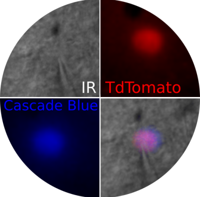
Connection detection
Connections were identified from manual inspection of the postsynaptic response aligned to the presynaptic spike. Excitatory and inhibitory connections could be observed in both voltage and current clamp at a holding potential that increased the driving force for each connection class. Weak connections were detectable by averaging hundreds of postsynaptic responses.
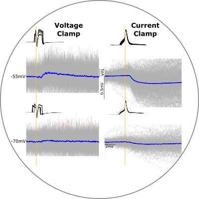
Connection characterization
Resting-state synaptic strength, rise/decay kinetics, and depth of short-term plasticity were calculated from curve fits of postsynaptic responses.
More on connection characterization
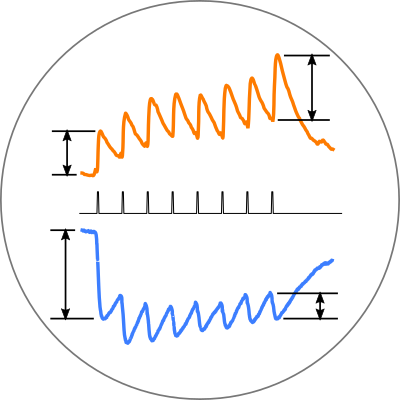
Quality control
Data passed through multiple quality control filters as part of the analysis workflow.

Learn about Synaptic Physiology Experimental Methods Experimental Protocol with comprehensive guides and examples from Allen Institute for Brain Science.
Experimental Stimuli
During a single experiment, a stereotyped set of stimuli were delivered to recorded cells to characterize the strength, kinetics, and short-term plasticity of synaptic connections. Each stimulus was delivered to cells in turn while recording the response from all other cells. Each stimulus train consisted of eight pulses to induce short-term plasticity (induction) followed by a delay and four pulses to measure recovery from dynamic effects. The frequency of pulses and delay were varied to measure these effects on synaptic connections. There was a 15 second delay between each stimulus to allow the cells to fully recover from stimulation. A separate set of stimuli were delivered to characterize the intrinsic properties of cells.
Stimulus Frequencies
A variety of stimulus frequencies were used, each with a 250 ms delay between the eight induction pulses and four recovery pulses.

Recovery Delays
For the 50 Hz stimulus, a range of recovery delays were interposed between the eight induction pulses and four recovery pulses to evaluate the time course of recovery from short-term effects.

Mixed Frequency Stimulus
The "mixed frequency" stimulus was composed of eight pulses delivered at 30Hz immediately followed by 30 pulses whose intervals were a random resequencing of 29 exponentially increasing intervals between 5 and 100ms. The intervals were fixed across sweeps and experiments. This stimulus allowed us to explore a wider range of stimulus frequencies that could be used to inform our model.
Stimulus Trials
Each stimulus, one frequency with one delay or mixed frequency, was repeated at least five times with a 15 second rest period between repeated trials. Spikes were recorded in the presynaptic cell along with postsynaptic responses.

Cell Intrinsic Stimuli
Long, sustained stimuli were delivered to each cell to measure intrinsic properties as well as quantify electrical synapses in current clamp. Intrinsic features were extracted from these stimuli using the IPFX package.
Subthreshold, mostly hyperpolarizing, stimuli were used to measure properties such as input resistance and sag. This stimulus set was initiated with a pulse at -20 pA while keeping the neuron at -70 mV. The voltage response to each current step was measured online and successive current steps were titrated to target response voltages of -68, -72, -75, -80, and -85 mV so as to reliably activate Ih when present.

Suprathreshold, depolarizing stimuli were delivered to measure spiking properties. These stimuli started at rheobase and increased 25 pA for 6 intervals.
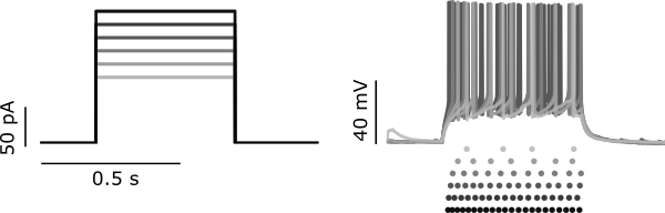
A 15-second sinusoidal chirp that increased in frequency from 0.2 to 40 Hz. The amplitude was targeted to evoke a response magnitude that measured ~10 mV from peak to trough.

Learn about Synaptic Physiology Experimental Methods Cell Class Targeting with comprehensive guides and examples from Allen Institute for Brain Science.
Cell Classification
Cell subclass was characterized by expression of a transgenic reporter(mouse) as well as by morphological properties (mouse and human). Cells were assigned to a target layer during the experiment followed by an annotated cortical layer during morphological analysis.
Transgenic Classification
Double, triple, and quadruple transgenic mice were used to label subclasses of excitatory and inhibitory cells. In triple and quadrupletransgenics, two distinct subclasses could be labeled with different reporters(typically TdTomato and EGFP). See the Transgenic Characterization for a complete description of the transgenic drivers and reporters.
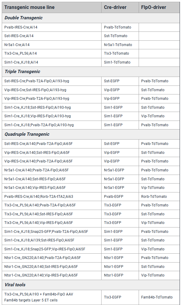
Morphological Classification
Biocytin filled cells were imaged at 63x magnification to measure morphological features such as spiny-ness, soma shape, and axon and dendritic length. More than 3000 mouse cells and 700 human cells received morphological analysis.
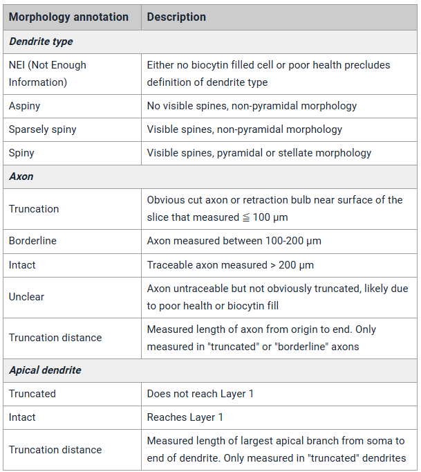
Layer Annotation
During the experiment we assigned a target layer to each cell as well as recorded the relative position of the cell within the slice. These cell positions were then mapped onto the biocytin and DAPI stained slice. When both annotated cortical layers, and cell positions were labeled on a slice these cells automatically received a "cortical layer" based on where the center of a cell was in relation to layer boundaries. We were able to assign cortical layers to more than 9000 mouse cells and 1400 human cells. Cells could be assigned a cortical layer even in the absence of biocytin as long as the position of the cells was recorded during the experiment.
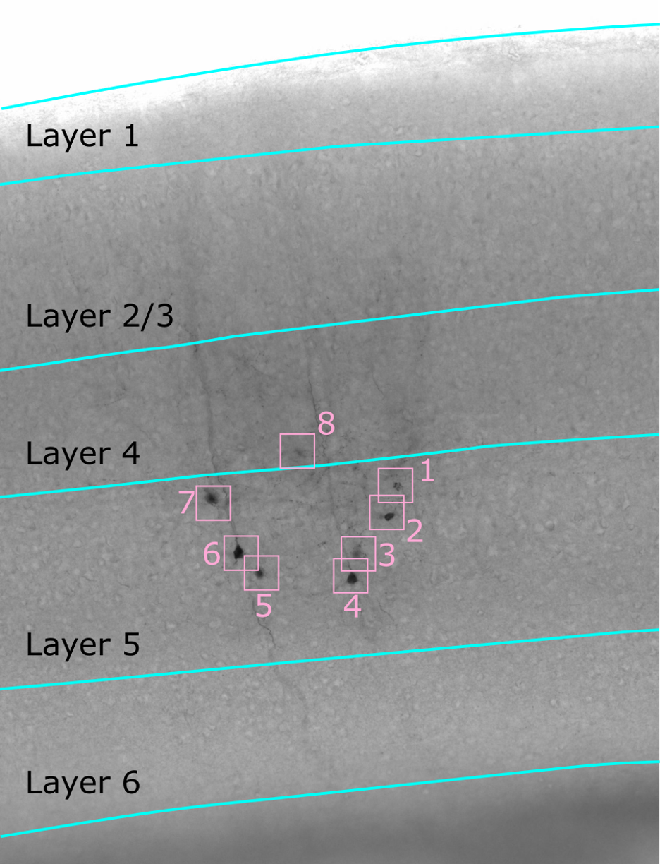
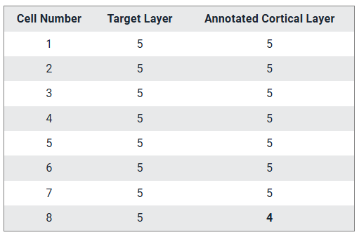
Learn about Synaptic Physiology Experimental Methods with comprehensive guides and examples from Allen Institute for Brain Science.
The Synaptic Physiology Dataset was generated with a standardized, large-scale approach using in vitro multipatch electrophysiology. This allowed us to explore connectivity among a diverse set of neuronal subclasses. Below is a workflow describing how this dataset was acquired; more detailed information can be found in our publications Seeman, Campagnola et al. 2018 and Campagnola, Seeman et al. 2022. Once data was collected it was processed through our Analysis Workflow.
Cell class targeting
Cre-/FlpO- transgenic breeding drove fluorescent reporter expression in two cell subclasses within the same mouse enabling targeted recording between them. Human excitatory cells were identified by morphology and cortical depth.
More on transgenic mouse lines

Acute cortical slices
Slices from adult (P40-P60) mouse primary visual cortex or human (18-75 years) frontotemporal cortex were prepared and held in artificial cerebrospinal fluid (aCSF) warmed to 32oC. The aCSF typically contained physiological levels (1.3 mM) of calcium.
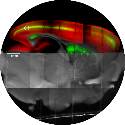
Octopatching
In each slice, up to eight neurons were recorded simultaneously, allowing for probing of up to 56 potential synaptic connections. Cells were recorded in voltage and current clamp mode at two holding potentials to identify excitatory and inhibitory connections.
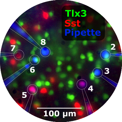
Experimental protocol
A variety of stimuli were delivered to each recorded cell in turn to characterize the strength, kinetics, and short-term plasticity of identified synapses. Synaptic stimuli consisted of trains of eight pulses at frequencies ranging from 10 - 200 Hz, followed by four pulses with a variable delay. Additional stimuli were delivered to measure intrinsic cell features.
More on the experimental protocol
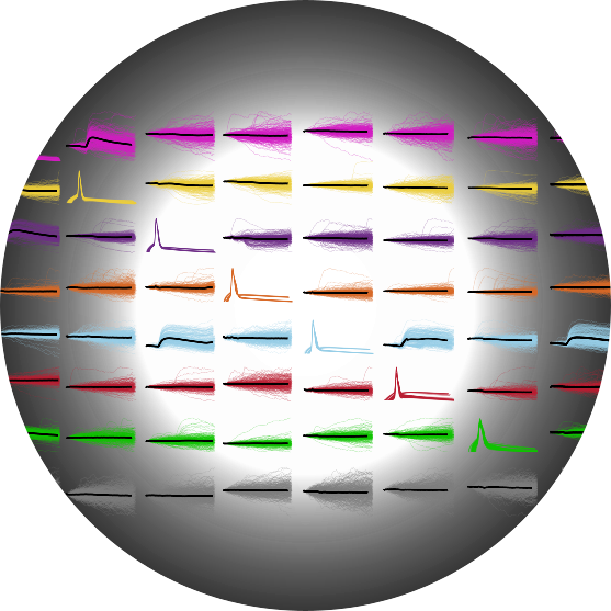
Morphological annotation
Recorded cells were filled with biocytin, and slices were fixed and stained. Layer boundaries were identified from DAPI staining. Biocytin-filled cells received an annotated layer as well as general morphologic characterization, including spiny-ness and axon and dendrite length.
More on morphological annotation
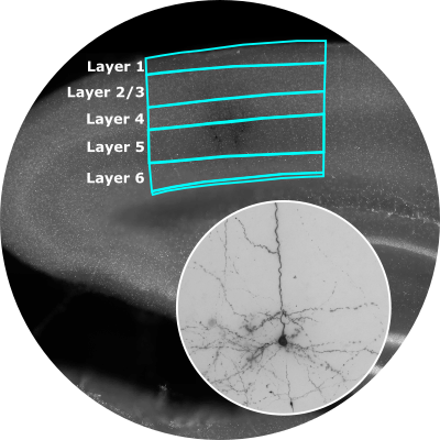
More Support Resources
Have a specific question or need more help? Check out our Community Forum
Become part of a supportive community created by scientists for scientists. Find answer to your own questions and help your colleagues use brain-map resources to their full extend with Community Forum's diverse content.