Tutorials

Thank you! Your submission has been received!

Oops! Something went wrong while submitting the form.

Onboarding

Download a file manifest for all female chimpanzees from Ed Lein’s - UM1MH130981 BICAN grant

Learn to download file manifests for female chimpanzee brain data from the BICAN grant. Access primate neuroscience research datasets.

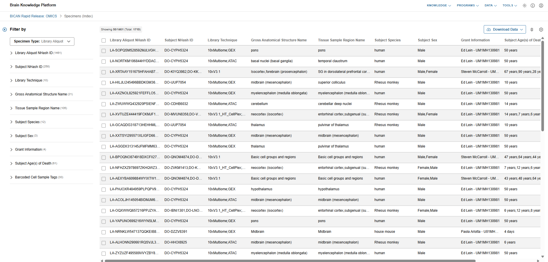
Step 1: I open the BICAN Rapid Release specimen viewer and get a general overview by scrolling around.

I review the overall BICAN specimen list and get an overview of the available library aliquots and donors.

Step 2: I use filters to reduce the list to only the grant that I’m interested in.

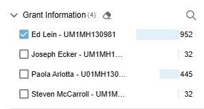
I’m a scientist doing research on non-human primates, particularly chimpanzees, and I closely follow the efforts by the Human and Mammalian Brain Atlas (HMBA) consortium within BICAN.

I filter down to only specimens from Ed Lein’s - UM1MH130981 grant as I know they fit my focus area. I see that 952 specimens are currently available from the grant.

Step 3: I filter further by species & sex.

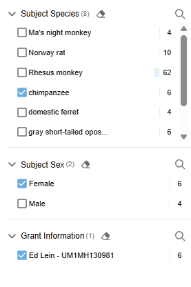
I’m looking to expand on my current data that is short on female chimpanzee specimens. I set additional filters for species = chimpanzee and sex = female. I see that 6 specimens currently match these criteria.

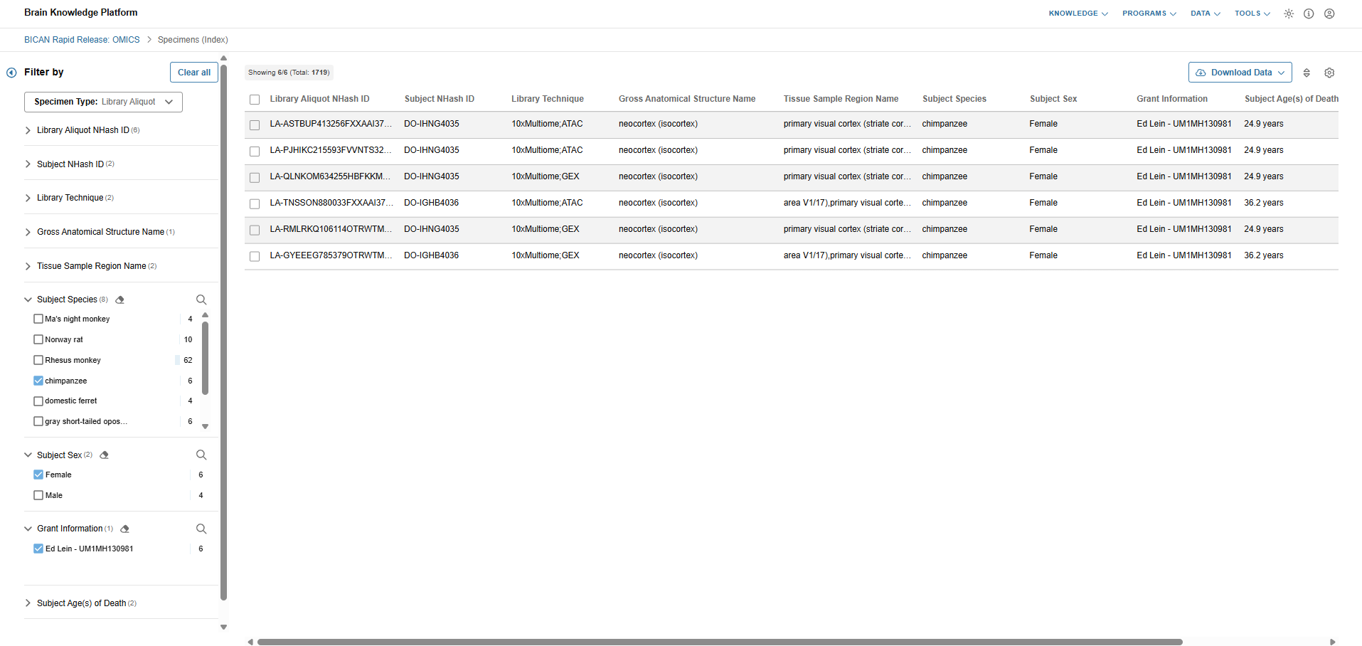
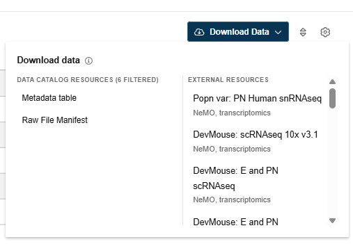
Step 4: I download the subset specimen metadata & file manifest and review them.

After reviewing the specimen metadata in the Data Catalog, I decide that they suitable for my purpose and download the metadata and file manifest for offline processing.

It includes 32 files for each library aliquot.

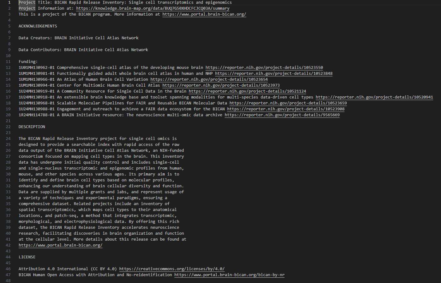
I review the documentation that comes with the file manifest and know how to access the fastq files at the archives.

Step 5: I access the fastq files at NeMO archive

Using the provided documentation, I access the fastq files at NeMO archive.

Learn More

Onboarding

Use BKP file manifest to access BICAN data at NeMO archive

Learn to access BICAN consortium data at NEMO Archive using BKP file manifests. Efficiently download large-scale brain research datasets.

Manifest download and formatting

Scientists can download a project’s file manifest from its specimens viewer in the BKP’s Data Catalog.

Example: Download the BICAN rapid release file manifest

Access the Project’s specimen viewer at https://knowledge.brain-map.org/data/BUQ7G50XHDCFCJCQ03A/specimens.
Filters down to a relevant subset of specimens via the UI’s filter capabilities.
Click the download button.
Select “File Manifest” from the modal.
Note: The file manifest may include both familiar HTTPS locations as well as GCP release bucket path (“gs://”). The latter are associated with restricted access data. Files referenced by these paths can be downloaded by users only after NeMO grants them access following approval from the NIMH Data Archive (NDA).
Unzip the downloaded .zip archive to access the readme and manifest.csv. The manifest output will match the filters & results of the user interface.

Archive tools may require adjusting the manifest’s column names and order to access data.

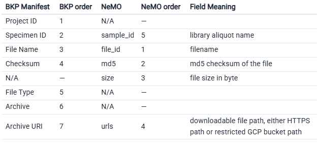
Note: You’ll need to manually add the size column. If there are no known values to fill, populate entries with a hyphen (“-”). Cells must not be empty.

You can then use the manifest in NeMO’s Portal-Client tool. See below for further details.

‍

NeMO: Rapid Release Collections and Data Access

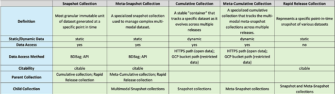
Introduction to Rapid Release Collection Types

The Rapid Release in BICAN is the immediate dissemination of high-quality, raw, and initial-processed -omics data (such as single-cell transcriptomics and epigenomics) to the public, typically within one calendar quarter (3 months) of its generation. It enables researchers to begin secondary analyses, develop new computational tools, or validate their own findings against the newest available brain cell maps.

NeMO utilizes specialized Snapshot, Cumulative, and Rapid Release collections to ensure the data released remains accessible and citable as data evolves.

Snapshot Collections (static)

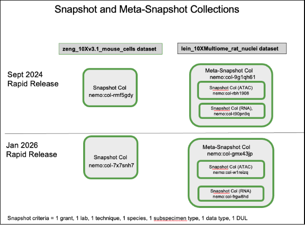
A “Snapshot” collection is the most granular immutable unit of dataset generated at a specific point in time defined by a unique combination of seven criteria: grant, lab, technique, species, subspecimen type, data type, and data use limitation (DUL). A new snapshot collection with a nemo identifier is created for files if the collection defined by the seven criteria was not part of the previous Rapid Release. Additionally, a snapshot collection is generated with a new NeMO identifier each time a Rapid Release occurs when there are new or modified files within that specific dataset. However, if no new data is included for a particular snapshot collection, the same collection identifier from the previous release is linked to the new Rapid Release. Please refer to ‘Diagram 1’ below. The files associated with these collections are packaged as BDBags for standardized data transfer. Each snapshot collection has a dedicated landing page that includes metadata associated with the data in the collection (such as taxa, modality, assay, technique, grant number, protocols, open or restricted data access etc.), a link to the BDBag, a specific data citation, and a link to the parent cumulative collection landing page. The landing page can be identified as a snapshot collection based on the collection name, which includes the prefix “BICAN__Snapshot”. The pages are hosted at assets.nemoarchive.org. To access the landing page for a specific collection in a web browser, append the NeMO identifier (‘col’ or ‘dat’ identifier) to the end of the URL, example: https://assets.nemoarchive.org/collection/nemo:col-7x7snh7.

A “Meta-Snapshot” collection is a specialized snapshot collection used to manage complex multi-modal dataset, such as Multiome datasets (e.g., RNA-seq and ATAC-seq performed on the same cells). These are “collections of snapshot collections” created at a specific point in time. A meta-snapshot collection is a parent for member snapshot collection. Please refer to ‘Diagram 1’ below. Its landing page contains a list of member snapshot collection landing page links, also including a “bag of bag” which is a parent BDBag packaged with child snapshot collection BDBags. The landing page can be identified as a meta-snapshot collection based on the collection name, which includes the prefix “BICAN__MetaSnapshot”. Example: https://assets.nemoarchive.org/collection/nemo:col-myr9nn1, is a multiome meta-snapshot collection landing page containing links to specific RNA-seq snapshot collection and an ATAC-seq snapshot collection generated for Jan, 2026 rapid release cycle. Each snapshot and meta-snapshot collection is a comprehensive aggregate, encompassing all data captured from the initial aliquot submission through the moment of collection generation.

Please refer to the section “Accessing Rapid Release Data” for downloading data associated with snapshot and meta-snapshot collections.

Diagram 1:

Cumulative Collections (dynamic)

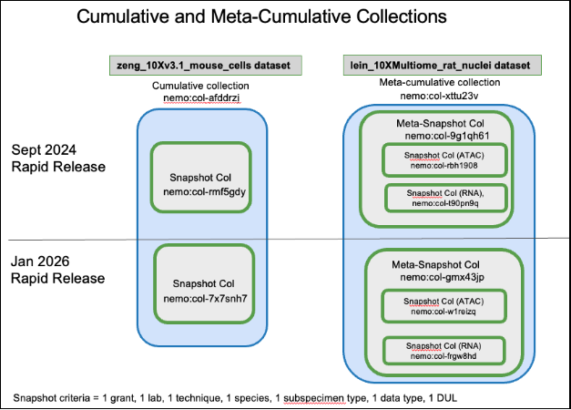
A “Cumulative” collection acts as a stable “container” that tracks a specific dataset as it evolves across multiple releases. It represents a “collection of collections”, where the members are all the individual static snapshot collections defined by a unique combination of seven criteria produced over various Rapid Release cycles. Please refer to ‘Diagram 2’ below. Unlike snapshot collection NeMO identifiers, cumulative collection identifiers don’t change as new Rapid Releases occur. The cumulative collection landing page provides a chronological list of individual static snapshot collection landing page links. They provide a persistent entry point for researchers to find the most current version of a dataset or view its history. They don’t contain BDBag links but provide links to the HTTPS location for accessing open data or the GCP release bucket path (“gs://”) for restricted data. The pages are hosted at assets.nemoarchive.org. To access the landing page for a specific collection in a web browser, append the NeMO identifier (‘col’ or ‘dat’ identifier) to the end of the URL, example: https://assets.nemoarchive.org/nemo:col-afddrzj. The landing page can be identified as a cumulative collection based on the collection name, which includes the prefix “BICAN__Cumulative”.

A “Meta-Cumulative” collection is a specialized cumulative collection that tracks the multi-modal meta-snapshot collections across multiple releases. It tracks the evolution of the member meta-snapshot collections across various Rapid Release cycles, ensuring that researchers can always find the latest multi-modal data through a single, persistent identifier. Similar to a standard cumulative collection, the meta-cumulative identifier remains constant across releases and don’t contain BDBag links but provide direct links to the HTTPS location for accessing open data or the GCP release bucket path (“gs://”) for restricted data. Please refer to ‘Diagram 2’ below. Example:https://assets.nemoarchive.org/col-iefmnby.

Diagram 2:

Rapid Release Collection (static)

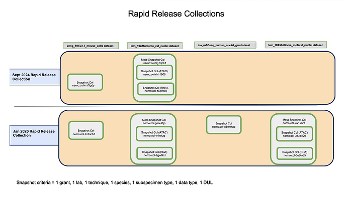
A “Rapid Release” collection represents a specific point-in-time snapshot of various datasets i.e., temporal grouping of all data released during a specific window of time. Each rapid release collection is composed of multiple unique static snapshot and meta-snapshot collections generated during that period. A new persistent rapid release NeMO identifier is generated with every rapid release. Each rapid release has a dedicated landing page including links to member snapshot collection landing pages. The landing page does not include a BDBag, nor does it provide HTTPS or GCP release bucket paths. Please refer to ‘Diagram 3’ below.

Diagram 3:

Overview of Collection Types

Data Collections available through Rapid Releases

All data collections released through the two Rapid Releases are publicly accessible. All collections from the September, 2024 Rapid Release contain open-access files available for free download. Except for two collections, all other January 2026 Rapid Release collections containing open-access data are freely available for download. The two exceptions contain restricted human fastq files, which can be accessed only upon approval from the NIMH Data Archive (NDA).

Here are the collection NeMO identifiers associated with Sept, 2024 and Jan, 2026 Rapid Releases.

Accessing Rapid Release Data

The following options are available for accessing Rapid Release data:

Landing Pages

Snapshot and Meta-snapshot collection landing pages:
Snapshot and meta-snapshot collection landing pages (https://assets.nemoarchive.org/api/collection/<nemo_identifier>) provide links to downloadable BDBags (an archive file containing downloadable file paths). To retrieve files, users must install the BDBag software. Detailed instructions for installing the tool and downloading files are available in the BDBag documentation. More information is available here. Each snapshot collection links to a single BDBag that includes a file metadata manifest listing all files available for download along with their associated metadata. A key metadata field in this manifest is the “library_aliquot_nhash_id”, a unique identifier for a library aliquot generated by the NIMP. This identifier can be used to retrieve donor and specimen metadata from the Brain Knowledge Platform’s (BKP) Data Catalog Specimen table and from NIMP via their APIs.

Meta-snapshot collection (eg: multiome) landing pages provide links to a master BDBag (a “bag of bags”). This master BDBag contains individual child BDBags, one for each snapshot collection included in the meta-snapshot. Each child BDBag includes its own file metadata manifest.

Open data BDBags: The BDBags linked in collections with open data contain downloadable HTTPS file paths.
Restricted data BDBags: The BDBags linked in collections with restricted data have GCP bucket file paths (gs://). Files referenced by these paths can be downloaded by users only after NeMO grants them access following approval from the NIMH Data Archive (NDA).

Cumulative and Meta-cumulative collection landing pages:

The cumulative and meta-cumulative collection landing pages do not contain links to BDBags but contain HTTPS paths for open access data and GCP bucket path (gs://) for restricted data. Restricted files referenced by GCP bucket paths (gs://) can be downloaded by users only after NeMO grants them access following approval from the NIMH Data Archive (NDA).

Rapid release collection landing page:
Files cannot be downloaded directly from this page. To access the data, users must navigate to each child snapshot collection landing page for accessing the files via a BDBag or NeMO API.

NeMO API endpoints

The NeMO API enables users to access and download data associated with grants, projects, subjects, samples (including libraries and aliquots), collections (including publications), and files. Both landing pages and API endpoints support metadata retrieval using NeMO identifiers as well as NIMP NHASH identifiers. API resources are available at https://assets.nemoarchive.org and do not require user authentication. Only publicly accessible metadata are displayed through the landing pages and APIs. Please refer to the detailed documentation on using the NeMO APIs to retrieve collection data.

Files associated with both snapshot and meta-snapshot collections can be retrieved using NeMO API endpoints. For collections containing restricted data, the file endpoints return restricted GCP bucket file paths, however, files can be downloaded only after the user has been granted access to the corresponding bucket. Please refer to the documentation describing the NIMH Data Archive (NDA) approval process for obtaining bucket access through NeMO.

Example 1: Retrieving files associated with a snapshot collection (nemo:col-a06sk1r) using paginated file endpoint

https://assets.nemoarchive.org/api/collection/nemo:col-a06sk1r/files?page=1&page_size=100

Example 2: Retrieving files associated with a meta-snapshot collection (nemo:col-myr9nn1).

Retrieve the two child snapshot collection endpoint URLs under meta-snapshot collection using collection endpoint.
‍https://assets.nemoarchive.org/api/collection/nemo:col-myr9nn1
Retrieve files associated with each snapshot collection using paginated file endpoint
‍https://assets.nemoarchive.org/api/collection/nemo:col-0onu0di/files?page=1&page_size=100 (ATAC dataset)
‍https://assets.nemoarchive.org/api/collection/nemo:col-o29aa39/files?page=1&page_size=100 (RNA dataset)

HTTPS location

The open access BICAN data are released at https://data.nemoarchive.org/. Grant specific data can be accessed by navigating through the data directory structure. The top-level (root) directory is organized by program. Within each program, data are further organized by grant, lab, modality, subspecimen type, technique, species, data type and aliquot name. Please note that the HTTPS location contains files released during the continuous release process (i.e., data automatically released after an embargo period ends). Consequently, some files may not be included in a Rapid Release collection.

Individual files can be downloaded directly from the browser by right-clicking the file and selecting “Copy” or “Save link as.” For downloading via command line, use any online tools that support http downloads such as Wget or cURL. Only cumulative and meta-cumulative collections with open access data are linked with HTTPS file locations.

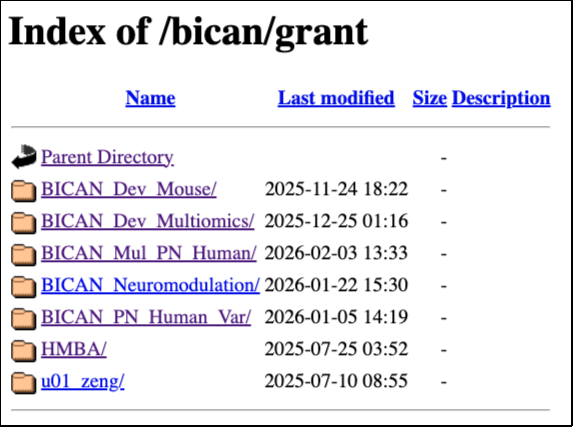
HTTPS location of BICAN data: https://data.nemoarchive.org/bican/grant/

Accessing NeMO Collections from Allen’s Brain Knowledge Platform (BKP)

There are two ways of finding NeMO collection data at Brain Knowledge Platform Data Catalog:

NeMO Collections linked in BKP Project Pages
Metadata search and file manifest retrieval from specimen table of BKP’s Data Catalog

NeMO Collections linked in BKP Project Pages

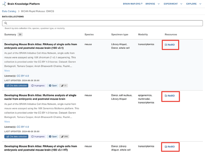
The NeMO collection landing page URLs are linked in each collection listed in “DATA COLLECTIONS” section in the project page - “BICAN Rapid Release Inventory: Single cell transcriptomics and epigenomics”. Click on the “NEMO” links to navigate to the corresponding collection landing pages where you will find links to collection BDBag and HTTPS path for file download. Refer to the document with details on downloading files using a BDBag. Details on accessing files from HTTPS links are in the section “HTTPS location” of this document. Allen Institute’s documentation on finding data for collections is here.

Metadata Search and File Manifest Retrieval from Specimen table of BKP’s Data Catalog

A tutorial on searching the metadata and downloading a file manifest from Specimen Table of BKP’s Data Catalog is posted for users reference here- “Download a file manifest for all female chimpanzees from Ed Lein’s - UM1MH130981 BICAN grant".

The file manifest downloaded from Data Catalog containing the HTTPS file paths can be used as an input into the Portal-Client tool to download the files after reformatting the manifest. Instructions can be found here in the Allen Brain Map Community Forum.

Please email nemo@som.umaryland.edu if you have any issues/suggestions/comments.

‍

Learn More

Onboarding

Finding AAVs for targeting Cholinergic cell populations in the striatum

Discover how to find AAV vectors for targeting cholinergic neurons in the striatum. Learn viral vector selection for precise cell targeting.

As a scientist doing research on the Basal Ganglia, I’m looking for viral genetic tools that allow me to specifically target cell types in the striatum for an upcoming set of experiments.

I use the Genetic Tools Atlas from the Allen Institute to explore whether Allen scientists have publicly shared suitable tools.

‍

Step 1: I open the Genetic Tools Atlas and get a general overview by scrolling around.

I review the provided experiment metadata. I see that at a glance there are several enhancer-adeno-associated viruses (AAVs) targeting the striatum but also ones for many other brain regions.

‍

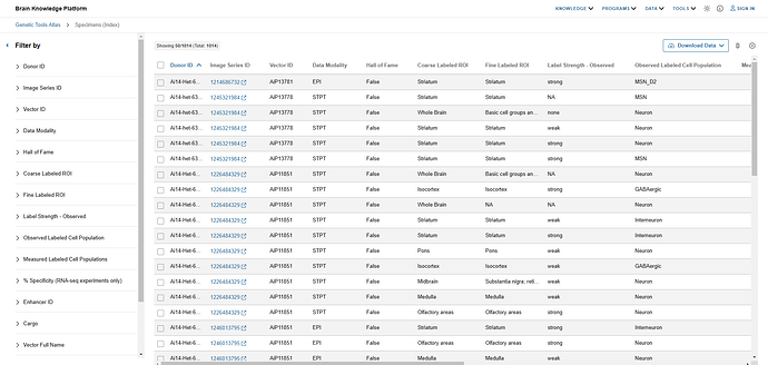
Step 2: I use filters to reduce the list to only experiments that target the striatum.

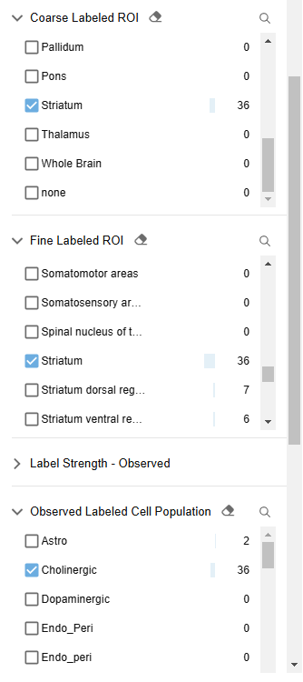
I open the filter panel and find the “Coarse Labeled ROI” filters. I scroll down and select the checkbox next to “Striatum“. I see that there are 372 results that match my query.

‍

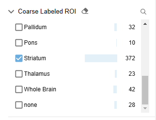
Step 3: I filter further to a “finer labeled ROI” & cell type of interest.

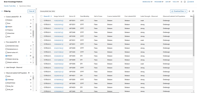
I apply an additional filter to narrow the data to a fine labeled ROI of “Striatum“ and an observed labeled cell population of “Cholinergic“. I’ve narrowed down my search to 36 highly relevant experiments.

‍

Step 4: I review “Hall of Fame” entries and related image data

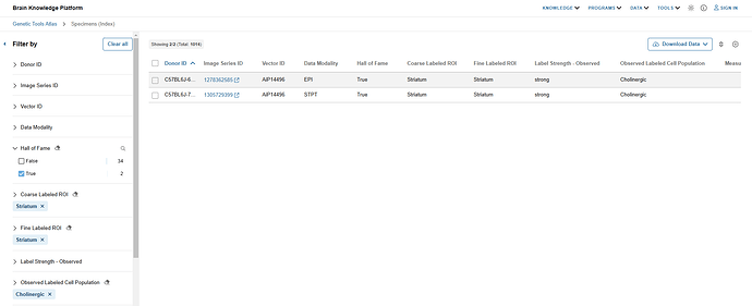
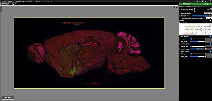
I notice that 2 results use AAVs that were designated as particularly notable, i.e. “Hall of Fame”. I review their EPI & STPT image data. I use Neuroglancer to see how these enhancers are expressed in my regions and cell populations of interest.

Useful Hot-Keys for Neuroglancer:

“ctrl + scroll” zoom
“R” and “E” rotate
“Z” locks to the nearby “straight” orientation
“scroll” move through volume for STPT images
“Shift + scroll” fast move through volume for STPT images

See the dedicated Neuroglancer documentation for more details.

‍

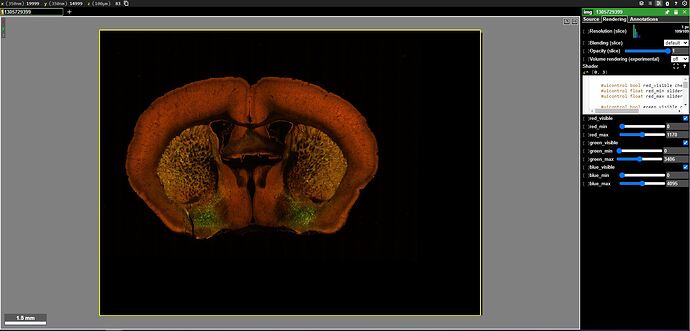
Step 5: I consider the enhancer suitable for my purposes and order it on Addgene - Vector ID lookup

The expression pattern meets my expectations and I decide to use it in future experiments.

I go to http://addgene.org . I type in the Vector ID “AiP14496“ I received from Genetic Tools Atlas and hit the Search button.

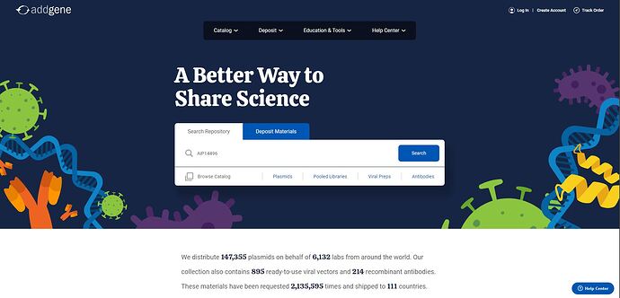
The results return one relevant enhancer:

I click into the enhancer entry to access further details and ordering information.

‍

Step 6: I explore non “Hall of Fame” entries and their image data

I explore the other results and find AiP13038 and its related image data. I use Neuroglancer to see how these enhancers are expressed in my regions and cell populations of interest. I note that its Addgene ID is listed directly in the Genetic Tools Atlas.

‍

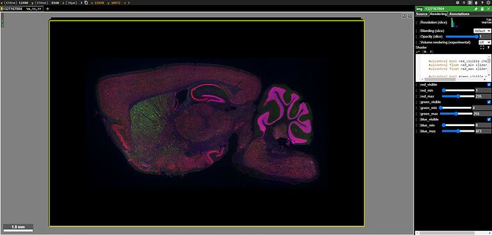
Step 7: I consider the enhancer suitable for my purposes and order it on Addgene - Addgene ID lookup

I go to addgene.org. I type in the enhancer ID “191720“ I received from Genetic Tools Atlas and hit the Search button.

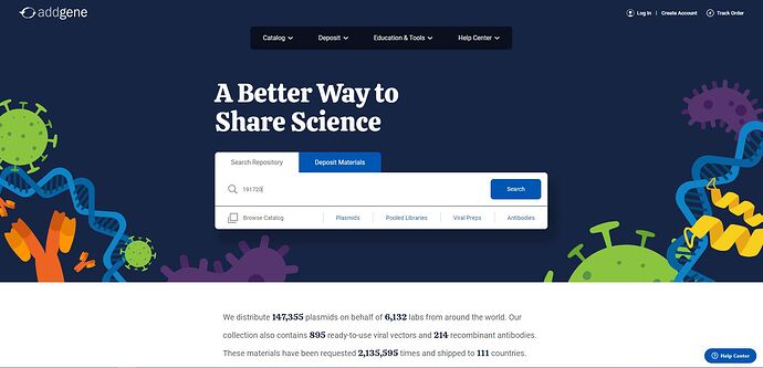
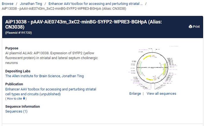
The results return one relevant enhancer:

I click into the enhancer entry to access further details and ordering information.

‍

Learn More

Onboarding

Guided exploration of ASAP-PMDBS data in the ABC Atlas

Take a guided tour of ASAP-PMDB Parkinson's disease data in the ABC Atlas. Explore molecular profiles and pathology across brain regions.

Overview

The ASAP-PMDBS dataset consists of ~3 million cells from five source datasets, spanning nine brain regions, and various pathologies. These cells were integrated and clustered into 30 clusters. Click on the hyperlinks to view these cells and filters in the ABC Atlas.

‍

Using with the Whole Human Brain taxonomy

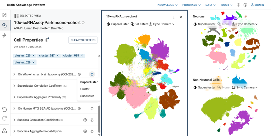
ASAP-PMDBS cells were mapped to the whole human brain (WHB) taxonomy (Siletti et al., 2023), which is hierarchical taxonomy of ~3.3 million cells (neurons and non-neuronal cells) with 31 superclusters, 461 clusters, and 3,313 subclusters spanning 105 anatomical dissections across the whole human brain. The 30 ASAP-PMDBS clusters were mapped at the WHB supercluster, cluster, and subcluster levels. Click on the hyperlinks to view the ASAP-PMDBS clusters in the ABC Atlas side-by-side with the WHB neuronal and non-neuronal cells.

To change the taxonomy level filter, click on the ink drop (🌢) next to "10x Whole human brain taxonomy" and click either supercluster, cluster, or subcluster.

‍

Using with the SEA-AD taxonomy

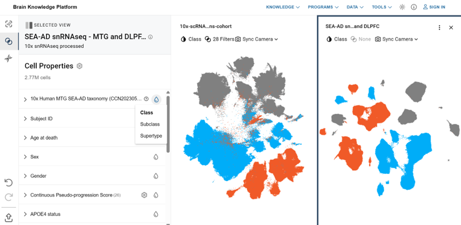
ASAP-PMDBS cells were also mapped to the Seattle Alzheimer’s Disease Brain Cell Atlas (SEA-AD) taxonomy (Gabitto and Travaglini et al., 2024), which contains ~1.4 million cells from the middle temporal gyrus (MTG) clustered into 3 classes, 24 subclasses, and 139 supertypes. The 30 ASAP clusters were mapped at the SEA-AD class, subclass, and supertype levels. Click on the hyperlinks to view the ASAP-PMDBS clusters in the ABC Atlas side-by-side with the SEA-AD cells.

To change the taxonomy level filter, click on the ink drop (🌢) next to "10x Human MTG SEA-AD taxonomy" and click either class, subclass, or supertype.

‍

Using with the SEA-AD MERFISH data

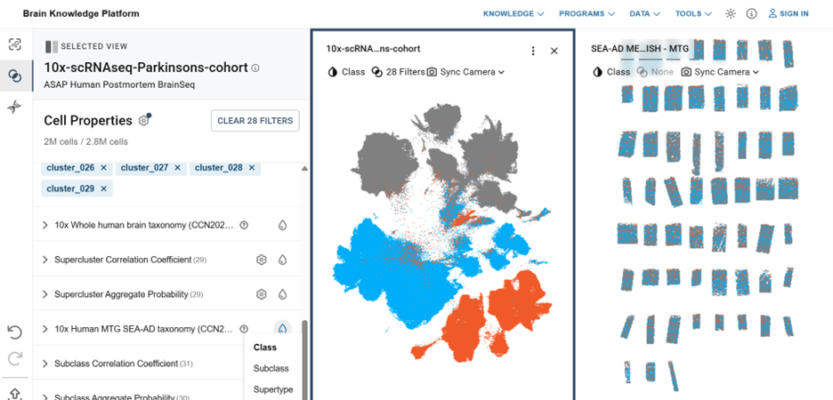
The SEA-AD taxonomy also features MERFISH spatial transcriptomic data from ~300k MTG cells from 24 of the SEA-AD donors. These cells are included in the 3 classes, 24 subclasses, and 139 supertypes. The ASAP-PMDBS cells mapped to the SEA-AD taxonomy can be viewed side-by-side with the MERFISH SEA-AD data at the class, subclass, and supertype levels. Click on the hyperlinks to view the ASAP-PMDBS clusters in the ABC Atlas side-by-side with the SEA-AD MERFISH cells.

Learn More

Onboarding

Video

Allen Mouse Brain Atlas

Watch this complete video tutorial on Allen Mouse Brain Atlas. Learn gene expression search, ISH image viewing, and anatomical navigation.

YouTube Tutorial

Learn More

Video

Allen Brain Observatory

Watch this comprehensive video tutorial on using Allen Brain Observatory. Learn to navigate visual coding datasets and analyze neural activity recordings.

YouTube Tutorials

‍

Two-photon dataset tutorial

‍

Neuropixels dataset tutorial

Learn More

Video

API

Atlas Drawing and Ontologies

Explore how brain atlases are created and organized through ontologies. Learn about anatomical structure hierarchies and classification systems.

A set of high resolution digital reference atlases have been created to provide neuroanatomical context to in situ hybridization, microarray, RNA-sequencing and axonal projection data.

From the API, you can:

Download the colorized and labeled atlas images
Download atlas graphics in SVG (scalable vector graphics) format
Download the underlying high resolution histological images
Download the associated structural ontology

The following Atlases are available through the API (click on Atlas ID to launch the interactive atlas viewer):

Atlas ID	Atlas Name	Image Type	Ontology	StructureGraph ID	GraphicGroupLabels
602630314	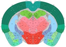“Adult Mouse, 3D Coronal”	“Atlas - Adult Mouse”	“Mouse Brain Atlas”	1	[28]
1	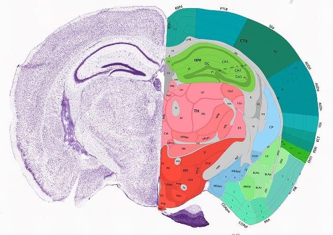“Mouse, P56, Coronal”	“Atlas - Adult Mouse”	“Mouse Brain Atlas”	1	[28,159226751]
2	“Mouse, P56, Sagittal”	“Atlas - Adult Mouse”	“Mouse Brain Atlas”	1	[28,159226751]
181276165	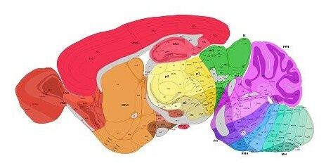“Developing Mouse, P56”	“Atlas - Developing Mouse”	“Developing Mouse Brain Atlas”	17	[32,167675952]
181276164	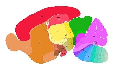“Developing Mouse, P14”	“Atlas - Developing Mouse”	“Developing Mouse Brain Atlas”	17	[32]
181276162	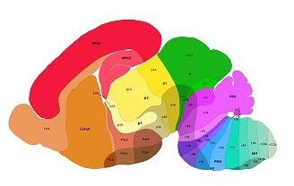“Developing Mouse, P4”	“Atlas - Developing Mouse”	“Developing Mouse Brain Atlas”	17	[32]
181276160	“Developing Mouse, E18.5”	“Atlas - Developing Mouse”	“Developing Mouse Brain Atlas”	17	[32]
181276151	“Developing Mouse, E15.5”	“Atlas - Developing Mouse”	“Developing Mouse Brain Atlas”	17	[32]
181276130	“Developing Mouse, E13.5”	“Atlas - Developing Mouse”	“Developing Mouse Brain Atlas”	17	[32]
181275741	“Developing Mouse, E11.5”	“Atlas - Developing Mouse”	“Developing Mouse Brain Atlas”	17	[32,126768961]
138322605	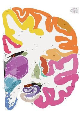“Human, 34 years, Cortex - Gyral”	“Atlas - Developing Human”	“Developing Human Brain Atlas”	16	[31,113753815,113753816,141667008]
265297126	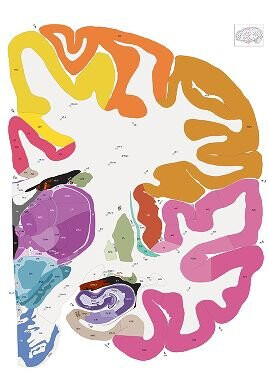“Human, 34 years, Cortex - Mod. Brodmann”	“Atlas - Developing Human Brodmann”	“Developing Human Brain Atlas”	16	[31,113753816,141667008,265297118]
3	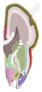“Human, 21 pcw”	“Atlas - Developing Human”	“Developing Human Brain Atlas”	16	[31,113753816,141667008]
287730656	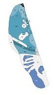“Human, 21 pcw - Brainstem”	“Atlas - Developing Human”	“Developing Human Brain Atlas”	16	[31,141667008]
138322603	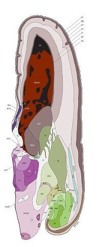“Human, 15 pcw”	“Atlas - Developing Human”	“Developing Human Brain Atlas”	16	[31,141667008]
265297125	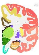"Human Brain Atlas Guide "	“Atlas - Human”	“Human Brain Atlas”	10	[265297119,266932194,266932196,266932197]

‍

Downloading Atlas Images And Graphics

The sections for each Atlas come from a single AtlasDataSet (child class of SectionDataSet) and single Specimen. Typically, only a subset of AtlasImages (child class of SectionImage) is used for the reference atlas. An “annotated” image is identified by the SubImage “annotated” attribute and the corresponding image type. Please note that multiple line example RMA queries on this page use the “+” character to represent spaces for browser compatibility.

Examples:

“Atlas - Adult Mouse” images for the “Mouse, P56 Coronal” atlas

‍

http://api.brain-map.org/api/v2/data/query.xml?criteria=model::AtlasImage, 
rma::criteria, 
[annotated$eqtrue], 
atlas_data_set(atlases[id$eq1]), 
alternate_images[image_type$eq'Atlas+-+Adult+Mouse'],
rma::options[order$eq'sub_images.section_number'][num_rows$eqall]

‍

“Atlas - Developing Human” images for the “Human, 34 years, Cortex - Gyral” atlas

‍

http://api.brain-map.org/api/v2/data/query.xml?criteria=model::AtlasImage, 
rma::criteria, 
[annotated$eqtrue], 
atlas_data_set(atlases[id$eq138322605]), 
alternate_images[image_type$eq'Atlas+-+Developing+Human'],
rma::options[order$eq'sub_images.section_number'][num_rows$eqall]

‍

Once the annotated images have been identified, the image ID can be used to download the colorized and labeled images using the Image Download Service and the vector graphics using the SVG Download Service.

Examples:

Download colorized and labeled image for one “Mouse, P56 Coronal” atlas image

‍

http://api.brain-map.org/api/v2/atlas_image_download/100960248?downsample=4&annotation=true

‍

View the vector graphics for one “Human, 34 years, Cortex - Gyral” atlas image

‍

http://api.brain-map.org/api/v2/svg/112360908?groups=31,113753815,113753816,141667008&downsample=8

‍

Download the vector graphics for one “Human, 34 years, Cortex - Gyral” atlas image

‍

http://api.brain-map.org/api/v2/svg_download/112360908?groups=31,113753815,113753816,141667008&downsample=8

‍

Structures And Ontologies

In the API, a Structure represents a neuroanatomical region of interest. Structures are grouped into Ontologies and organized in a hierarchy or StructureGraph. With the exception of the “root” structure, each Structure has one parent and denotes a “part-of” relationship. Structures are assigned a color to visually emphasize their hierarchical position in the brain. See the Structure model page for listing of attributes and associations.

Major structural ontologies used in the Allen Brain Atlas Data Portal:

Ontology ID	Ontology Name	StructureGraph ID	Uses
1	“Mouse Brain Atlas”	1	Mouse Brain, Mouse Connectivity Reference Atlases, Brain Explorer, AGEA, Informatics quantification of ISH data, Informatics quantification of projection data, Search services
12	“Developing Mouse Brain Atlas”	17	Developing Mouse Brain, Reference Atlases, Brain Explorer, AGEA, Informatics quantification of ISH data, Search services
7	“Human Brain Atlas”	10	Human Brain, Annotation of microarray Sampling Sites, Brain Explorer, Heatmap and search services, “Hot spot” annotation of ISH data, Human Brain Atlas Guide
11	“Developing Human Brain Atlas”	16	Developing Human Brain, Reference Atlases, Annotation of RNA-sequencing and microarray Sampling Sites, Heatmap and search services, “Hot spot” annotation of ISH data
4	“Non-Human Primate Brain Atlas”	8	Non-Human Primate, Annotation of microarray Sampling Sites, Heatmap and search services, “Hot spot” annotation of ISH data
10	“Glioblastoma”	15	Glioblastoma, Human Glioblastoma RNASeq, Annotation of tumor features on H&E and ISH data, Annotation of RNA-Seq sampling sites

From the API, Structure and Ontology information can be downloaded in various formats.

Examples:

Download the “Human Brain Atlas” ontology as a CSV file

‍

http://api.brain-map.org/api/v2/data/query.csv?criteria=model::Structure, rma::criteria,[ontology_id$eq7], rma::options[order$eq%27structures.graph_order%27][num_rows$eqall]

‍

Download the “Mouse Brain Atlas” ontology as a hierarchically structured json file

‍

http://api.brain-map.org/api/v2/structure_graph_download/1.json

‍

Download the “Developing Human Brain Atlas” ontology as a hierarchically structured json file

‍

http://api.brain-map.org/api/v2/structure_graph_download/16.json

Learn More

API

Image-to-Image Synchronization

Master image-to-image synchronization for comparing brain atlas data. Navigate corresponding sections across multiple datasets simultaneously.

The following set of image synchronization services uses the image alignment results from the Informatics Data Processing Pipeline. Note: all locations on SectionImages are reported in pixel coordinates and all locations in 3-D ReferenceSpaces are reported in microns.

‍

Image-to_Atlas

For a specified Atlas, find the closest annotated SectionImage and (x,y) location as defined by a seed SectionImage and seed (x,y) location.

‍

Prototype

‍

http://api.brain-map.org/api/v2/image_to_atlas/[SectionImage.id].[xml|json]?x=[#]&y=[#]&z=[#]&atlas_id=[#]

‍

Example

For a seed location in SectionImage 68173101, locate the closest image and (x,y) position within the P56 coronal Atlas:

‍

http://api.brain-map.org/api/v2/image_to_atlas/68173101.xml?x=6208&y=2368&atlas_id=1

‍

Parameters

filename	Integer	Seed SectionImage for spatial sync.
file extension	String	XML or JSON format is specified as the file extension.
x	Float	x pixel coordinate of the seed location in the seed SectionImage.
y	Float	y pixel coordinate of the seed location in the seed SectionImage.
atlas_id	Integer	Target Atlas for image sync.

‍

Returns

XML or JSON document containing the following:

section_image_id	Closest annotated SectionImage to the seed SectionImage and pixel location.
section_number	Section number of the closest SectionImage.
x	Closest x pixel coordinate on the closest SectionImage.
y	Closest y pixel coordinate on the closest SectionImage.

‍

Image-to_Image

For a list of target SectionDataSets, find the closest SectionImage and (x,y) location as defined by a seed SectionImage and seed (x,y) pixel location.

‍

Prototype

‍

http://api.brain-map.org/api/v2/image_to_image/[SectionImage.id].[xml|json]?x=[#]&y=[#]&section_data_set_ids=[#,#,#...]

‍

Example

For seed location in SectionImage 68173101, locate the closest 3-D position in each input SectionDataSet.

‍

http://api.brain-map.org/api/v2/image_to_image/68173101.xml?x=6208&y=2368&section_data_set_ids=67810540,69782969

‍

Parameters

filename	Integer	Seed SectionImage for spatial sync.
file extension	String	XML or JSON format is specified as the file extension.
x	Float	x pixel coordinate of the seed location in the seed SectionImage.
y	Float	y pixel coordinate of the seed location in the seed SectionImage.
section_data_set_ids	Array	Comma delimited list of target SectionDataSet IDs for image sync.

‍

Returns

XML or JSON document containing the following for each SectionDataSet in the section_data_set_ids:

section_image_id	Closest SectionImage to the seed SectionImage and pixel location.
section_number	Section number of the closest SectionImage.
x	Closest x pixel coordinate on the closest SectionImage.
y	Closest y pixel coordinate on the closest SectionImage.

‍

Image-to-Image 2-D

For a list of target SectionImages, find the closest (x,y) location as defined by a seed SectionImage and seed (x,y) location.

‍

Prototype

‍

http://api.brain-map.org/api/v2/image_to_image_2d/[SectionImage.id].[xml|json]?x=[#]&y=[#]&section_image_ids=[#,#,#...]

‍

Example

For a seed location in SectionImage 68173101, locate the closest 2-D position in each input SectionImage:

‍

http://api.brain-map.org/api/v2/image_to_image_2d/68173101.xml?x=6208&y=2368&section_image_ids=68173103,68173105,68173107

‍

Parameters

filename	Integer	Seed SectionImage ID for image sync.
file extension	String	XML or JSON format is specified as the file extension.
x	Float	x pixel coordinate of the seed location in the seed SectionImage.
y	Float	y pixel coordinate of the seed location in the seed SectionImage.
section_image_ids	Array	Comma delimited list of target SectionImage IDs for image sync.

‍

Returns

XML or JSON document containing the following for each SectionImage in the section_image_ids:

x	Closest x pixel coordinate to the seed location.
y	Closest y pixel coordinate to the seed location.

‍

Reference-To-Image

For a list of target SectionDataSets, find the closest SectionImage and (x,y) location as defined by a (x,y,z) location in a specified ReferenceSpace.

‍

Prototype

‍

http://api.brain-map.org/api/v2/reference_to_image/[ReferenceSpace.id].[xml|json]?x=[#]&y=[#]&z=[#]&section_data_set_ids=[#,#,#...]

‍

Example

For a 3-D seed location in the P56 ReferenceSpace, locate the closest image and (x,y) location for each input SectionDataSet.

‍

http://api.brain-map.org/api/v2/reference_to_image/10.xml?x=6085&y=3670&z=4883&section_data_set_ids=68545324,67810540

‍

Parameters

filename	Integer	Seed ReferenceSpace for spatial sync.
file extension	String	XML or JSON format is specified as the file extension.
x	Float	x coordinate (in microns) of the seed location in the seed ReferenceSpace.
y	Float	y coordinate (in microns) of the seed location in the seed ReferenceSpace.
z	Float	z coordinate (in microns) of the seed location in the seed ReferenceSpace.
section_data_set_ids	Array	Comma delimited list of target SectionDataSets IDs for image sync.

‍

Returns

XML or JSON document containing the following for each SectionDataSet in the section_data_set_ids:

section_image_id	Closest SectionImage to the seed ReferenceSpace and location.
section_number	Section number of the closest SectionImage.
x	Closest x pixel coordinate to the seed location.
y	Closest y pixel coordinate to the closest SectionImage.

‍

Image-To-Reference

For a specified SectionImage and (x,y) location, return the (x,y,z) location in the ReferenceSpace of the associated SectionDataSet.

‍

Prototype

‍

http://api.brain-map.org/api/v2/image_to_reference/[SectionImage.id].[xml|json]?x=[#]&y=[#]

‍

Example

For a location in SectionImage 68173101, return the (x,y,z) position in the associated ReferenceSpace.

‍

http://api.brain-map.org/api/v2/image_to_reference/68173101.xml?x=6208&y=2368

‍

RMA query to return the associated ReferenceSpace:

‍

http://api.brain-map.org/api/v2/data/query.xml?criteria=
model::SubImage, rma::criteria,[id$eq68173101],
rma::include,data_set, 
rma::options[only$eq'data_sets.id,data_sets.reference_space_id,sub_images.id']

‍

Parameters

filename	Integer	SectionImage.id.
file extension	String	XML or JSON format is specified as the file extension.
x	Float	x pixel coordinate on the specified SectionImage.
y	Float	y pixel coordinate on the specified SectionImage.

‍

Returns

XML or JSON document containing the (x,y,z) location in the associated ReferenceSpace.

x	x coordinate (in microns) in the associated ReferenceSpace.
y	y coordinate (in microns) in the associated ReferenceSpace.
z	z coordinate (in microns) in the associated ReferenceSpace.

‍

Structure-To-Image

For a list of target structures, find the closest SectionImage and (x,y) location as defined by the centroid of each Structure.

‍

Prototype

‍

http://api.brain-map.org/api/v2/structure_to_image/[SectionDataSet.id].[xml|json]?structure_ids=[#,#,#...]

‍

Example

For each Structure in the input list, locate the closest image and (x,y) location in SectionDataSet 68545324:

‍

http://api.brain-map.org/api/v2/structure_to_image/68545324.xml?structure_ids=315,698,1089,703,477,803,512,549,1097,313,771,354

‍

Parameters

filename	Integer	ID of the closest SectionImage to the 3-D centroid of the structure.
file extension	String	XML or JSON format is specified as the file extension.
structure_ids	Array	List of target Structures for sync.

‍

Returns

XML or JSON document containing the following for each Structure in the structure_ids:

section_image_id	Closest SectionImage to the 3-D centroid of the structure.
section_number	Section number of the closest SectionImage.
x	Closest x pixel coordinate of the closest SectionImage.
y	Closest y pixel coordinate of the closest SectionImage.

Learn More

API

Downloading 3-D Expression Grid Data

Learn to download 3-D expression grid data as NRRD files. Access voxel-level gene expression values for computational brain analysis.

Downloading 3-D Expression Grid Data

‍

Download 3-D expression grid data packaged into a compressed archive file (.zip).

‍

Prototype

‍

http://api.brain-map.org/grid_data/download/[SectionDataSet.id]&include=[images]

‍

Examples

Download the 200um density volume for the Mouse Brain Atlas SectionDataSet 69816930:

‍

http://api.brain-map.org/grid_data/download/69816930

‍

Download the 200um energy and intensity volumes for Mouse Brain Atlas SectionDataSet 69816930:

‍

http://api.brain-map.org/grid_data/download/183282970?include=energy,intensity

‍

Download the energy volume for the Mouse Brain Atlas’ coronal Adora2a experiment.

First, search for relevant experiments’ IDs (SectionDataSets):

‍

http://api.brain-map.org/api/v2/data/query.xml?criteria= model::SectionDataSet, rma::criteria,[failed$eq'false'],products[abbreviation$eq'Mouse'],plane_of_section[name$eq'coronal'],genes[acronym$eq'Adora2a']

‍

Then, download the energy volume for each of the experiments’ IDs:

‍

http://api.brain-map.org/grid_data/download/72109410?include=energy

‍

Parameters

ID	Integer	ID of the desired SectionDataSet.
include	String (optional)	Explicitly choose the desired image volumes. Valid volumes are energy, density, and intensity. Supply multiple volumes in a comma-delimited list (e.g. “include=energy,density,intensity”). By default, only energy is returned.

‍

Response

Zip file (.zip) containing a folder filled with the default files (data_set.xml, energy.mhd, energy.raw) or the requested data volumes.

data_set.xml	XML file with details regarding the specimen and images that is only returned if the volumes parameter is null.
energy.mhd	A simple text header file in MetaImage format describing the volume. This file is returned by default if the volumes parameter is null.
energy.raw	A raw uncompressed float (32-bit) little-endian volume representing average expression energy per voxel. A value of “-1” represents no data. This file is returned by default if the volumes parameter is null.
density.mhd	A simple text header file in MetaImage format describing the volume.
density.raw	A raw uncompressed float (32-bit) little-endian volume representing average expression density per voxel. A value of “-1” represents no data.
intensity.mhd	A simple text header file in MetaImage format describing the volume.
intensity.raw	A raw uncompressed float (32-bit) little-endian volume representing average expression intensity per voxel. A value of “-1” represents no data.
injection.mhd	A simple text header file in MetaImage format describing the volume.
injection.raw	A raw uncompressed float (32-bit) little-endian volume representing the proportion of pixels within each voxel that were within the manually annotated injection site.

‍

Downloading 3-D Projection Grid Data

Download 3-D projection grid data packaged into a compressed .nrrd image.

‍

Prototype

http://api.brain-map.org/grid_data/download_file/[SectionDataSet.id]&image=[image]&resolution=[resolution]

‍

Examples

Download the 100um density volume for the Mouse Connectivity Atlas SectionDataSet 181777177:

‍

http://api.brain-map.org/grid_data/download_file/181777177

‍

Download the 25um injection_fraction volume for Mouse Connectivity Atlas SectionDataSet 181777177:

‍

http://api.brain-map.org/grid_data/download_file/181777177?image=injection_fraction&resolution=25

‍

Parameters

ID	Integer	ID of the desired SectionDataSet.
image	String (optional)	Explicitly choose the desired image volume. Valid volumes are projection_density, projection_energy, injection_fraction, injection_density, injection_energy, and data_mask.
resolution	Integer (optional)	Available resolutions for projection data are 10, 25, 50, and 100 (in microns).

‍

Response

The response will be a single 32-big floating point Nrrd image named for the requested image type and resolution. If no image is specified, the density volume is returned. If no resolution is specified, 100um resolution is assumed.

projection_density	Density of projecting signal (number of projecting pixels / volume)
projection_energy	Density of projecting signal multiplied by total signal intensity
injection_fraction	Fraction of pixels belonging to the injection site
injection_density	Density of projecting signal for pixels belonging to the injection site
injection_energy	Injection density multiplied by total signal intensity for pixels belonging to the injection site
data_mask	Binary image where a value of ‘1’ indicates that greater than 50% of a grid voxel contains valid data.

Learn More

API

Video

Allen Human Brain Atlas

Follow this video guide to master Allen Human Brain Atlas. Learn to search genes, explore expression patterns, and navigate human brain anatomy.

YouTube Tutorial

Learn More

Video

API

Downloading a WellKnownFile

Discover how to download .well-known files from Allen Institute resources. Access metadata and configuration information for data integration.

The WellKnownFile Download Service returns files. Examples include Agilent output files from the Human Brain Microarray product and RNA Sequencing output files from the Developing Human Developing Human Transcriptome product.

‍

Prototype

‍

http://api.brain-map.org/api/v2/well_known_file_download/[WellKnownFile.id]

‍

Example

Download the Human Brain Microarray Atlas “raw” Agilent output files associated with Donor H0351.2001 and the DG Structure.

First, search for all WellKnownFiles associated with Donor H0351.2001 and the Structure DG:

‍

http://api.brain-map.org/api/v2/data/query.xml?criteria= model::Sample,
rma::criteria,microarray_data_set(products[abbreviation$eq'HumanMA'],specimen(donor[name$eq'H0351.2001'])),structure[acronym$eq'DG'],
rma::include,microarray_slides(well_known_files)

‍

Next, iterate through the WellKnownFile elements, building URLs by appending the WellKnownFile.download_link value to “http://api.brain-map.org”:

‍

http://api.brain-map.org/api/v2/well_known_file_download/3486

‍

Parameters

filename String WellKnownFile.id identifying the file to download.

‍

Returns

The file represented by the specified WellKnownFile.id. Several file formats may be returned by this service.

Learn More

API

Downloading and Displaying SVG

Learn to download and display SVG graphics from Allen Brain Atlas. Work with scalable anatomical diagrams for research and presentations.

The SVG download service returns annotations associated with the specified SectionImage as scalable vector graphics (SVG). Examples of annotations that can be retrieved include hot spots and drawings of Structure boundaries on AtlasImages. Add the “groups=” parameter and specify one or more GraphicGroupLabel.id delimited by commas to filter the types of SVG returned.

‍

Prototype

‍

http://api.brain-map.org/api/v2/svg_download/[SectionImage.id]?groups=[#, #, #...]

‍

Examples

Find Atlases that have AtlasImages annotated with Structure boundaries, and the relevant GraphicGroupLabel.ids:

‍

http://api.brain-map.org/api/v2/data/query.xml?criteria= model::Atlas,
rma::include,graphic_group_labels[name$il'Atlas*'],
rma::options[only$eq'atlases.id,atlases.name,graphic_group_labels.id']

‍

Download a list of AtlasImages from the “Mouse, P56 Coronal” Atlas (id=1) that have Structure boundary annotations (GraphicGroupLabel.id=28):

‍

http://api.brain-map.org/api/v2/data/query.csv?criteria= model::AtlasImage,
rma::criteria,atlas_data_set(atlases[id$eq1]),graphic_objects(graphic_group_label[id$eq28]),
rma::options[tabular$eq'sub_images.id'][order$eq'sub_images.id'] &num_rows=all&start_row=0

‍

Download the structure boundary annotations (GraphicGroupLabel.id=28) for an AtlasImage (id=100960033) as a file (.svg):

‍

http://api.brain-map.org/api/v2/svg_download/100960033?groups=28

‍

Display SVG in most browsers:

‍

http://api.brain-map.org/api/v2/svg/100960033?groups=28

‍

Parameters

filename	Integer	SectionImage.id identifying the SVG to download.
groups	list of Group.id (optional)	Filter the Groups to include in the SVG

‍

Returns

SVG as either a downloaded file or displayed in the browser.

Learn More

API

Downloading an Ontology's Structure Graph

Download ontology structure graphs showing brain anatomy hierarchies. Access anatomical structure relationships and organizational data.

Allows downloading of an Ontology’s StructureGraph as a JSON or XML document. Review the list of Atlas Drawings and Ontologies to determine the relevant StructureGraph’s ID.

‍

Prototype

‍

http://api.brain-map.org/api/v2/structure_graph_download/[StructureGraph.id].[xml|json]

‍

Examples

Download the Mouse Brain Atlas Ontology’s StructureGraph (StructureGraph id=1):

‍

http://api.brain-map.org/api/v2/structure_graph_download/1.json

‍

Download the Human Brain Atlas Ontology’s StructureGraph (StructureGraph id=10):

‍

http://api.brain-map.org/api/v2/structure_graph_download/10.json

‍

Parameters

filename	Integer	StructureGraph.id
file extension	String	.xml or .json format.

‍

Returns

A hierarchical XML or JSON document containing each of the Structures in the requested StructureGraph with the following:

parent_id	ID of the parent Structure.
children	1…n descendants of the Structure

Learn More

API

Downloading an Image

Learn to download high-resolution brain images from Allen Institute. Access ISH images, atlas sections, and microscopy data with quality options.

Download whole or partial two-dimensional images from the Allen Institute with the Image and AtlasImage Download Services.

‍

Image Download Service

The Image download service serves whole and partial two-dimensional images presented on the Allen Brain Atlas Web site. Some images can be downloaded with expression or projection data. Glioblastoma images’ color block and boundary data can also be downloaded.

‍

Prototype

‍

http://api.brain-map.org/api/v2/image_download/[SubImage.id]?downsample=[#]&quality=[#]&view=[expression|projection|tumor_feature_annotation|tumor_feature_boundary]

‍

Examples

Download a downsampled SectionImage of one sagittal section from the Mouse Brain Pdyn SectionDataSet:

‍

http://api.brain-map.org/api/v2/image_download/69750516?downsample=4

‍

Download a downsampled expression mask for a SectionImage of one sagittal section from the Mouse Brain Pdyn SectionDataSet:

‍

http://api.brain-map.org/api/v2/image_download/69750516?downsample=4&view=expression

‍

Download a region of interest at full resolution from the same sagittal SectionImage:

‍

[type or paste code here](http://api.brain-map.org/api/v2/image_download/69750516?left=6174&top=2282&width=1000&height=1000)

‍

Download SectionImage 71592261 downsampled 3 times with 50% image quality:

‍

http://api.brain-map.org/api/v2/image_download/71592261?downsample=3&quality=50

‍

Download the downsampled SectionImage 126862583 with projection:

‍

http://api.brain-map.org/api/v2/projection_image_download/126862583?downsample=4&view=projection

‍

Determine the default range values for a Mouse Connectivity Projection experiment by referring to its associated Equalization model (red_lower=0, red_upper=923, green_lower=0, green_upper=987, blue_lower=0, blue_upper=4095), then download one of its downsampled SectionImages:

‍

http://api.brain-map.org/api/v2/data/SectionDataSet/100141599.xml?include=equalization,section_images 
http://api.brain-map.org/api/v2/image_download/102146167?range=0,923,0,987,0,4095&downsample=4

‍

Download the color block or color boundary image designating tissue features of Glioblastoma tumor:

‍

http://api.brain-map.org/api/v2/image_download/311175878?downsample=4&view=tumor_feature_annotation
http://api.brain-map.org/api/v2/image_download/311174547?downsample=4&view=tumor_feature_boundary

‍

Find the closest NISSL image to SectionImage 71592261 and download it:

First, search for the closest NISSL image:

‍

http://api.brain-map.org/api/v2/data/query.xml?criteria= 
model::SectionImage, 
rma::criteria,[id$eq71592261], rma::include,associates(data_set(treatments[name$eq'NISSL']))

‍

Second, download the NISSL image using the Associate.id:

‍

http://api.brain-map.org/api/v2/image_download/71592412

‍

Download all of the sagittal images in the Mouse Brain Atlas for the gene Adora2a at full resolution.

First, search for relevant experiments’ IDs (SectionDataSets):

‍

http://api.brain-map.org/api/v2/data/query.xml?criteria= \
model::SectionDataSet, 
rma::criteria,[failed$eq'false'],products[abbreviation$eq'Mouse'],plane_of_section[name$eq'sagittal'],genes[acronym$eq'Adora2a']

‍

Second, retrieve a list of all images for one of the experiments (SectionImages):

‍

http://api.brain-map.org/api/v2/data/query.xml?criteria= 
model::SectionImage, 
rma::criteria,[data_set_id$eq70813257]

‍

Finally, iterate through the list of images and call the SectionImage Download Service with their IDs:

‍

http://api.brain-map.org/api/v2/image_download/70679088

‍

Parameters

filename	Integer	SectionImage.id identifying the image to download.
view	String (optional)	* Set the value to expression to retrieve the specified SectionImage’s expression mask image. Set the value to tumor_feature_annotation to retrieve the color block image for a Glioblastoma SectionImage. Set the value to tumor_feature_boundary to retrieve the color boundary image for a Glioblastoma SectionImage. Set the value to projection to retrieve the specified SectionImage with projection.
downsample	Integer (optional)	The number of times to downsample the original image. For example, ‘downsample=1’ halves the number of pixels of the original image both horizontally and vertically. Specifying ‘downsample=2’ quarters the height and width values.
quality	Integer (optional)	The jpeg quality of the returned image. This must be an integer from 0, for the lowest quality, up to as high as 100. If it is not specified, it defaults to the highest quality.
left	Integer (optional)	Index of the leftmost column of the region of interest, specified in full-resolution (largest tier) pixel coordinates. SectionImage.x is the default value.
top	Integer (optional)	Index of the topmost row of the region of interest, specified in full-resolution (largest tier) pixel coordinates. SectionImage.y is the default value.
width	Integer (optional)	Number of columns in the output image, specified in tier-resolution (desired tier) pixel coordinates. SectionImage.width is the default value. It is automatically adjusted when downsampled.
height	Integer (optional)	Number of rows in the output image, specified in tier-resolution (desired tier) pixel coordinates. SectionImage.height is the default value. It is automatically adjusted when downsampled.
range	Array (optional)	Filter to specify the RGB channels. The range parameter consists of 6 comma delimited integers that define the lower (0) and upper (255) bound for each channel in red-green-blue order (i.e. “range=0,1500,0,1000,0,4095”). The default range values can be determined by referring to the following fields on the Equalization model associated with the SectionDataSet: red_lower, red_uppper, green_lower, green_upper, blue_lower, blue_upper. For more information, see the “Image Controls” section of the Allen Mouse Brain Connectivity Atlas: Projection Dataset help topic.

‍

Returns

A jpeg file of the requested image.

‍

AtlasImage Download Service

The AtlasImage download service serves whole and partial two-dimensional images with annotations presented on the Allen Brain Atlas Web site.

‍

Prototype

‍

http://api.brain-map.org/api/v2/atlas_image_download/[AtlasImage.id]?downsample=[#]&quality=[#]&annotation=[true|false]&atlas=[#]

‍

Examples

Download the downsampled AtlasImage 100883869 with annotations:

‍

http://api.brain-map.org/api/v2/atlas_image_download/100883869?downsample=4&annotation=true

‍

Request P56 Mouse Brain Atlas’ annotations:

‍

http://api.brain-map.org/api/v2/atlas_image_download/100883869?downsample=4&annotation=true&atlas=2

‍

Request P56 Developing Mouse Brain Atlas’ annotations:

‍

http://api.brain-map.org/api/v2/atlas_image_download/100883869?downsample=4&annotation=true&atlas=181276165

‍

Download all of the Mouse, P56 Sagittal Atlas’ Nissl images.

First, review the list of current Atlas Drawings and Ontologies to determine the Mouse, P56 Sagittal Atlas’ ID (Atlas id=2).

Second, retrieve a list of the Mouse, P56 Sagittal Atlas’ Nissl images (Atlas id=2):

‍

http://api.brain-map.org/api/v2/data/query.xml?criteria= 
model::Atlas, 
rma::criteria,[id$eq2], 
rma::include,atlas_data_sets(atlas_images(treatments))

‍

Finally, iterate through the list of AtlasImages and call the AtlasImage Download Service to download the Nissl images:

‍

http://api.brain-map.org/api/v2/atlas_image_download/100883771

‍

Parameters

filename	Integer	AtlasImage.id identifying the image to download.
annotation	Boolean (optional)	Set the value to true to retrieve the specified AtlasImage with annotations.
atlas	Integer (optional)	Specify the desired Atlas.ID for the annotations. The P56 Adult Mouse Brain Atlas and Developing Mouse Brain Atlas share a common AtlasDataSet, so the Atlas.ID should be specified.
downsample	Integer (optional)	The number of times to downsample the original image. For example, ‘downsample=1’ halves the number of pixels of the original image both horizontally and vertically. Specifying ‘downsample=2’ quarters the height and width values.
quality	Integer (optional)	The jpeg quality of the returned image. This must be an integer from 0, for the lowest quality, up to as high as 100. If it is not specified, it defaults to the highest quality.
left	Integer (optional)	Index of the leftmost column of the region of interest, specified in full-resolution (largest tier) pixel coordinates. SectionImage.x is the default value.
top	Integer (optional)	Index of the topmost row of the region of interest, specified in full-resolution (largest tier) pixel coordinates. SectionImage.y is the default value.
width	Integer (optional)	Number of columns in the output image, specified in tier-resolution (desired tier) pixel coordinates. SectionImage.width is the default value. It is automatically adjusted when downsampled.
height	Integer (optional)	Number of rows in the output image, specified in tier-resolution (desired tier) pixel coordinates. SectionImage.height is the default value. It is automatically adjusted when downsampled.

‍

Returns

A jpeg file of the requested image.

Learn More

API

Onboarding

MapMyCells Use case: single cell genomics in mouse

Use MapMyCells to map mouse single-cell genomics data to Allen taxonomies. Classify your cells using reference transcriptomics data.

Overview

Click here to download the full R notebook for your own use

MapMyCells enables mapping of single cell and spatial trancriptomics data sets to a whole mouse brain taxonomy. The taxonomy is derived and presented in “A high-resolution transcriptomic and spatial atlas of cell types in the whole mouse brain” (https://www.biorxiv.org/content/10.1101/2023.03.06.531121v1), and we encourage you to cite this work if you use MapMyCells to transfer these labels to your date. This R workbook illustrates a common use case for the MapMyCells facility (https://knowledge.brain-map.org/mapmycells/process/) and follow up analyses. The query data included in this document are from the paper “The cell type composition of the adult mouse brain revealed by single cell and spatial genomics” (https://doi.org/10.1101/2023.03.06.531307) from the Chen and Macosko labs, which also has a nice data exploration tool (Brain Cell Data Viewer; https://docs.braincelldata.org/).

‍

Prepare your workspace

‍

Install R and (optionally RStudio)

This example is run and R, which can be downloaded at CRAN (https://cran.r-project.org/). To run in R, just sequentially copy and paste the relevant code blocks into R. An easier alternative is to download RStudio here (https://posit.co/download/rstudio-desktop/) after downloading R. “.Rmd” files can be directly loaded into R studio and run.

‍

Prior to running any code, download the data:

To get started first download an example 10x library from the paper above. We choose data from primary motor cortex (MOp) to apply knowledge from the series of 2021 BICCN studies at https://www.biccn.org/cell-census-primary-motor-cortex. Extract the file below from the NeMO archive to your working directory: https://data.nemoarchive.org/biccn/grant/u19_huang/macosko_regev/transcriptome/sncell/10X_v2/mouse/processed/counts/pBICCNsMMrMOPi70470511Bd180328.mex.tar.gz Unzipping will produce a folder called “pBICCNsMMrMOPi70470511Bd180328” with three files: “Matrix.mtx”, “barcodes.tsv”, and “genes.tsv”. This is the standard output for a single 10X run (and other droplet-based methods), and data can be read in using standard R scripts. The MOP in the file name indicates that this particular library is from a primary motor cortex dissection.

Now you are ready to start R (or RStudio).

‍

Set the working directory

The next component of set up is to make sure your R working directory points to the data you are reading in.

# Uncomment line below and replace bracketed text with path to downloaded files.
#setwd("FILE_PATH")

‍

Load the relevant libraries

This workbook uses the libraries anndata and Seurat.

# Install Seurat and anndata if needed
list.of.packages <- c("Seurat", "anndata")
new.packages <- list.of.packages[!(list.of.packages %in% installed.packages()[,"Package"])]
if(length(new.packages)>0) install.packages(new.packages)

# Load Seurat and anndata
suppressPackageStartupMessages({
  library(Seurat)      # For reading droplet data sets and visualizing/comparing results
  library(anndata)     # For writing h5ad files 
})Warning: package ‘Seurat’ was built under R version 4.2.3Warning: package ‘anndata’ was built under R version 4.2.3options(stringsAsFactors=FALSE)

# Citing R libraries# citation("Seurat") 
# Note that the citation for any R library can be pulled up using the citation command. We encourage citation of R libraries as appropriate.

‍

With the above files in your current working directory and the above libraries loaded, the use case below can now be run.

‍

Analysis of a library

(If you already have an .h5ad file ready for upload, skip to step 4.)

A common use case for analysis of single cell/nucleus transcriptomics is to collect data from one (or more) ports of a droplet-based scRNA-seq run. After some QC steps, these are then clustered for defining cell types. This section describes how to start from a such a droplet-based sequencing run, transfer labels from mouse “10x scRNA-seq whole brain” data from the Allen Institute onto these cells using MapMyCells, and then visualize the results in a UMAP.

‍

1. Read library data into R

10x (and other droplet-based) output includes files for the cells (“barcodes.tsv”), the genes (“genes.tsv”), and the corresponding reads (“matrix.mtx”). These can be read into a sparse matrix in R with appropriate formatting using the function “Read10X”.

dataIn <- Read10X("pBICCNsMMrMOPi70470511Bd180328/")
dim(dataIn)[1]  27998 737280

‍

This reads in a data matrix with >700,000 columns as potential cells. However, this includes all of the empty wells.

‍

2. QC data

For demonstrative purposes, we will define all barcodes with >250 reads as interesting “cells”, but in a real experiment more careful QC is strongly encouraged.

dataQC <- dataIn[,colSums(dataIn)>250]
dim(dataQC)[1] 27998  3673

‍

This brings the input library down to a more reasonable ~3600 cells.

‍

3. Output to h5ad format

Now let’s output the QC’ed data matrix into an h5ad file and output it to the current directory for upload to MapMyCells. Note that in anndata data structure the genes are saved as columns rather than genes so we need to transpose the matrix first.

# Transpose data
dataQCt = Matrix::t(dataQC)

# Convert to anndata format
ad <- AnnData(
  X = dataQCt,
  obs = data.frame(group = rownames(dataQCt), row.names = rownames(dataQCt)),
  var = data.frame(type = colnames(dataQCt), row.names = colnames(dataQCt))
)

# Write to compressed h5ad file
write_h5ad(ad,'droplet_library.h5ad',compression='gzip')

# Check file size. File MUST be <500MB to upload for MapMyCells
print(paste("Size in MB:",round(file.size("droplet_library.h5ad")/2^20)))[1] "Size in MB: 14"

‍

If you have trouble accessing or running the previous block, check your Python accessibility in R and consider installing python as shown below. If you use Windows, you may be asked to install git before installing python, which can be accessed here: https://git-scm.com/download/win/.

library(reticulate)
version <- "3.9.12"
install_python(version)
virtualenv_create("my-environment", version = version)
use_virtualenv("my-environment")

‍

4. Assign cell types using MapMyCells

These next steps are performed OUTSIDE of R in the MapMyCells web application.

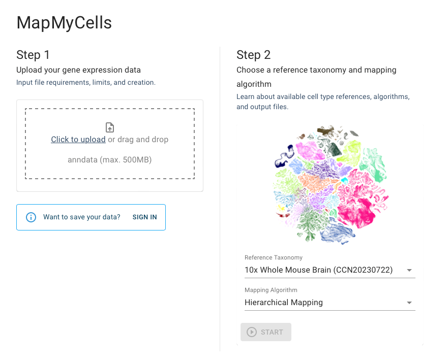
The steps to MapMyCells are as follows:

Go to (https://knowledge.brain-map.org/mapmycells/process/).
(Optional) Log in to MapMyCells.
Upload ‘droplet_library.h5ad’ to the site via the file system or drag and drop (Step 1).
Choose “10x Whole Mouse Brain (CCN20230722)” as the “Reference Taxonomy” (Step 2).
Choose the desired “Mapping Algorithm” (in this case “Hierarchical Mapping”).
Click “Start” and wait ~5 minutes. (Optional) You may have a panel on the left that says “Map Results” where you can also wait for your run to finish.
When the mapping is complete, you will have an option to download the “tar” file with mapping results. If your browser is preventing popups, search for small folder icon to the right URL address bar to enable downloads.
Unzip this file, which will contain three files: “validation_log.txt”, “[NUMBER].json”, and “[NUMBER].csv”. [NUMBER].csv contains the mapping results, which you need. The validation log will give you information about the the run itself and the json file will give you extra information about the mapping (you can ignore both of these files if the run completes successfully).
Copy [NUMBER].csv to your current working directory and rename it “droplet_library_mapping.csv”).
You can now go back to R and continue the script below.

‍

5. Read mapping results into R

Let’s now look at the output results from the hierarchical clustering algorithm. We can read this into R using read.csv, but note that the first four lines contain metadata that need to be skipped.

mapping <- read.csv("droplet_library_mapping.csv",comment.char="#")
head(data.frame(mapping))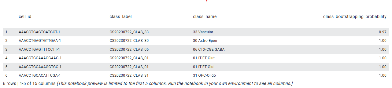

MapMyCells maps input cells to the taxonomy at four increasing levels of resolution from coarsest class, to intermediate subclass, and supertype, and finest cluster. In the mouse whole brain taxonomy there are 32 classes, 306 subclasses, 1,045 supertypes and 5,200 clusters.

The file consists of the following columns:

cell_id = the cell identifiers for your cells included in the initial h5ad files
class_label = the unique identifier for the best mapping class
class_name = the name of the best mapping class
class_bootstrapping_probability = fraction of bootstrapping runs that the cell mapped to the above class (higher numbers are better, with 1 being the best)
and similar fields for subclass, supertype, and cluster. For finest level cluster there is an additional field
cluster_alias = another unique identifier for the cluster

‍

6. Review top classes

As this library was selected from a dissection of primary motor cortex (MOp), we expect the majority of cells to map to cell types found in MOp. Let’s check!\

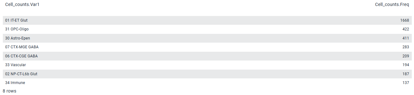
# View the top 8 classes
data.frame(Cell_counts=head(sort(table(mapping$class_name),decreasing=T),8))

‍

# What fraction of all cells does this represent
sum(t(t(head(sort(table(mapping$class_name),decreasing=T),8))))/length(mapping$class_name)[1] 0.9558944

‍

The 8 most common mapped classes representing >95% of cells are glutamatergic, GABA-ergic or non-neuronal types known to be present in MOp from many published studies.

‍

7. Visualize mapping results

To visualize the mapping results, we need both the mapping results and the original query cellxgene matrix for comparison. If this is not already read in, you can read it in from the anndata object uploaded to MapMyCells.

# Since the query data corresponds to dataQC above, we will call it dataQC again
dataQC_h5ad <- read_h5ad('droplet_library.h5ad')dataQC <- t(as.matrix(dataQC_h5ad$X))
rownames(dataQC) <- rownames(dataQC_h5ad$var)
colnames(dataQC) <- rownames(dataQC_h5ad$obs)

‍

Now let’s visualize the mapping results. We will do this by saving the data in a Seurat object with (modified) mapping results as metadata, running the standard pipeline for creating a UMAP in Seurat, and then color-coding each cell.

# Assign rare classes and subclasses as "other"
mapping$class_new <- mapping$class_name
mapping$class_new[!is.element(mapping$class_name,names(head(-sort(-table(mapping$class_name)),8)))] = "other"
mapping$subclass_new <- mapping$subclass_name
mapping$subclass_new[!is.element(mapping$subclass_name,names(head(-sort(-table(mapping$subclass_name)),20)))] = "other"

# Put row.names as data colnames and the order to match the data
rownames(mapping) <- mapping$cell_id
mapping <- mapping[colnames(dataQC),]

# Create the Seurat object
dataSeurat <- CreateSeuratObject(counts = dataQC, meta.data = mapping)

# Standard Seurat pipeline
dataSeurat <- NormalizeData(dataSeurat, verbose = FALSE)
dataSeurat <- FindVariableFeatures(dataSeurat, verbose = FALSE)
dataSeurat <- ScaleData(dataSeurat, verbose = FALSE)
dataSeurat <- RunPCA(dataSeurat, verbose = FALSE)
dataSeurat <- RunUMAP(dataSeurat, dims = 1:10, verbose = FALSE)

‍

‍Now let’s make the plot for classes!

DimPlot(dataSeurat, reduction = "umap", group.by="class_new", label=TRUE) + NoLegend()

‍

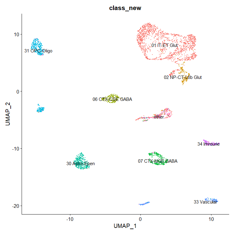
Here the data has not been clustered but rather the class assignments are assigned to the data in the UMAP. The alignment suggests that the label transfer works well. It’s worth noting that Seurat produces different UMAP configurations in different R environments, so your plot may not look exactly like this.

Now let’s make the plot where we color-code the same UMAP by subclass.

DimPlot(dataSeurat, reduction = "umap", group.by="subclass_new", label=TRUE) + NoLegend()

‍

‍

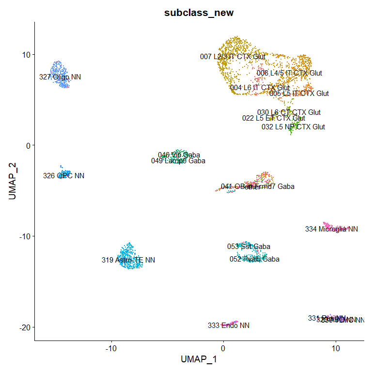
Once again, the subclasses shown largely segregate from one another without the need to apply clustering, suggesting this mapping works well even at higher resolutions. Scripts such as this can be used for visualizing and comparing mapping results.

To output the session information we write the command, which is useful for reproducibility, especially for more complex scripts.

sessionInfo()R version 4.2.2 (2022-10-31 ucrt)
Platform: x86_64-w64-mingw32/x64 (64-bit)
Running under: Windows 10 x64 (build 19045)

Matrix products: default

locale:
[1] LC_COLLATE=English_United States.utf8  LC_CTYPE=English_United States.utf8    LC_MONETARY=English_United States.utf8 LC_NUMERIC=C
[5] LC_TIME=English_United States.utf8

attached base packages:
[1] stats     graphics  grDevices utils     datasets  methods   base

other attached packages:
[1] anndata_0.7.5.6    SeuratObject_5.0.0 Seurat_4.4.0

loaded via a namespace (and not attached):
[1] Rtsne_0.16             colorspace_2.1-0       deldir_1.0-9           ellipsis_0.3.2         ggridges_0.5.4         rstudioapi_0.15.0       
[7] spatstat.data_3.0-3    farver_2.1.1           leiden_0.4.3           listenv_0.9.0          ggrepel_0.9.4          fansi_1.0.5            
[13] codetools_0.2-19       splines_4.2.2          R.methodsS3_1.8.2      knitr_1.45             polyclip_1.10-6        spam_2.10-0            
[19] jsonlite_1.8.7         ica_1.0-3              cluster_2.1.4          png_0.1-8              R.oo_1.25.0            uwot_0.1.16            
[25] shiny_1.7.5.1          sctransform_0.4.1      spatstat.sparse_3.0-3  compiler_4.2.2         httr_1.4.7             assertthat_0.2.1       
[31] Matrix_1.6-1.1         fastmap_1.1.1          lazyeval_0.2.2         cli_3.6.1              later_1.3.1            htmltools_0.5.6.1      
[37] tools_4.2.2            igraph_1.5.1           dotCall64_1.1-0        gtable_0.3.4           glue_1.6.2             RANN_2.6.1             
[43] reshape2_1.4.4         dplyr_1.1.3            Rcpp_1.0.11            scattermore_1.2        vctrs_0.6.4            spatstat.explore_3.2-5 
[49] nlme_3.1-163           progressr_0.14.0       lmtest_0.9-40          spatstat.random_3.2-1  xfun_0.40              stringr_1.5.0          
[55] globals_0.16.2         mime_0.12              miniUI_0.1.1.1         lifecycle_1.0.3        irlba_2.3.5.1          goftest_1.2-3          
[61] future_1.33.0          MASS_7.3-60            zoo_1.8-12             scales_1.2.1           promises_1.2.1         spatstat.utils_3.0-4   
[67] parallel_4.2.2         RColorBrewer_1.1-3     reticulate_1.34.0      pbapply_1.7-2          gridExtra_2.3          ggplot2_3.4.4          
[73] stringi_1.7.12         rlang_1.1.1            pkgconfig_2.0.3        matrixStats_1.0.0      lattice_0.22-5         ROCR_1.0-11            
[79] purrr_1.0.2            tensor_1.5             labeling_0.4.3         patchwork_1.1.3        htmlwidgets_1.6.2      cowplot_1.1.1          
[85] tidyselect_1.2.0       parallelly_1.36.0      RcppAnnoy_0.0.21       plyr_1.8.9             magrittr_2.0.3         R6_2.5.1               
[91] generics_0.1.3         withr_2.5.2            pillar_1.9.0           fitdistrplus_1.1-11    survival_3.5-7         abind_1.4-5            
[97] sp_2.1-1               tibble_3.2.1           future.apply_1.11.0    KernSmooth_2.23-22     utf8_1.2.4             spatstat.geom_3.2-7   
[103] plotly_4.10.3          grid_4.2.2             data.table_1.14.8      digest_0.6.33          xtable_1.8-4           tidyr_1.3.0           
[109] httpuv_1.6.12          R.utils_2.12.2         munsell_0.5.0          viridisLite_0.4.2

Learn More

Onboarding

MapMyCells Use case: single nucleus RNA-seq from human MTG

Map human MTG single nucleus RNA-seq data using MapMyCells. Classify cells against Allen human brain reference taxonomies.

Overview

Click here to download the full R notebook for your own use

MapMyCells enables mapping of single cell and spatial trancriptomics data sets to a human middle temporal gyrus (MTG) taxonomy. The taxonomy is derived and presented in “Integrated multimodal cell atlas of Alzheimer’s disease” (https://doi.org/10.1101/2023.05.08.539485), and we encourage you to cite this work if you use MapMyCells to transfer these labels to your data. It is also used throughout the web tools on SEA-AD.org. This R workbook illustrates a common use case for the MapMyCells facility (https://knowledge.brain-map.org/mapmycells/process/) and follow up analyses. The query data included in this document are from the paper “Conserved cell types with divergent features in human versus mouse cortex ” (https://doi.org/10.1038/s41586-019-1506-7) from the Allen Institute, which also has a nice data exploration tool (RNA-Seq Data Navigator; https://celltypes.brain-map.org/rnaseq/human/mtg).

‍

Prepare your workspace

‍

Install R and (optionally RStudio)

‍

Download the query data

As an example data set, we will use the a subset of the snRNA-seq dataset published in Hodge, et al. (2019), which has been conveniently packaged into an R library. (To see how one would perform this step from a 10X experiment, see the version of this tutorial for whole mouse brain.)

if(!is.element("hodge2019data",.packages(all.available = TRUE)))  # Install data package if not already installed
  devtools::install_github("AllenInstitute/hodge2019data")

‍

Set the working directory

The next component of set up is to make sure your R working directory points to the data you are reading in.

# Uncomment line below and replace bracketed text with path to downloaded files.
#setwd("FILE_PATH")

‍

Load the relevant libraries

This workbook uses the libraries anndata, Seurat, and hodge2019data.

# Install Seurat and anndata if needed
list.of.packages <- c("Seurat", "anndata")
new.packages <- list.of.packages[!(list.of.packages %in% installed.packages()[,"Package"])]
if(length(new.packages)>0) install.packages(new.packages)

suppressPackageStartupMessages({
  library(Seurat)        # For reading droplet data sets and visualizing/comparing results
  library(anndata)       # For writing h5ad files
  library(hodge2019data) # For the query data set
})

## Warning: package 'Seurat' was built under R version 4.2.3## Warning: package 'anndata' was built under R version 4.2.3options(stringsAsFactors=FALSE)

# Citing R libraries# citation("Seurat")
# Note that the citation for any R library can be pulled up using the citation command. We encourage citation of R libraries as appropriate.

‍

With the above libraries loaded, the use case below can now be run.

‍

Analysis of snRNA-seq data

(If you already have an .h5ad file ready for upload, skip to step 4.)

A common use case for analysis of single cell/nucleus transcriptomics is to collect data from several thousand cells, either though one (or more) ports of a droplet-based scRNA-seq run or using single well per cell SMART-Seq sequencing. After some QC steps, these are then clustered for defining cell types. This section describes how to start from such a data set, transfer labels from human “Human-MTG-10x_SEA-AD” data from the Allen Institute / SEA-AD onto these cells using MapMyCells, and then visualize the results in a UMAP.

‍

1. Read query data

With the data library loaded, these are already read in. We just rename for convenience.

dataIn <- data_Hodge2019        # These are the counts
annoIn <- metadata_Hodge2019    # These are the metadata (e.g., cluster assignments)
dim(dataIn)## [1] 36591  3357

‍

This reads in a data matrix with 3,357 nuclei.

‍

2. QC data

The above data has already been carefully QC’ed, and therefore a QC step is unnecessary. However, in a typical experiment a QC step would be needed at this point. For demonstrative purposes, we will define all barcodes with >250 reads as interesting “cells”, but in a real experiment more careful QC is strongly encouraged.

dataQC <- dataIn[,colSums(dataIn)>250]
dim(dataQC)## [1] 36591  3357

‍

This step retains all cells for this example, but in a droplet-based experiment it would typically bring the input library down from a huge number to a more reasonable number.

‍

3. Output to h5ad format

# Transpose data
dataQCt = Matrix::t(dataQC)

# Convert to anndata format
ad <- AnnData(  
  X = dataQCt,
  obs = data.frame(group = rownames(dataQCt), row.names = rownames(dataQCt)),
  var = data.frame(type = colnames(dataQCt), row.names = colnames(dataQCt))
)
  
# Write to compressed h5ad file
write_h5ad(ad,'Hodge2019.h5ad',compression='gzip')

# Check file size. File MUST be <500MB to upload for MapMyCells
print(paste("Size in MB:",round(file.size("Hodge2019.h5ad")/2^20)))## [1] "Size in MB: 73"

‍

library(reticulate)
version <- "3.9.12"
install_python(version)
virtualenv_create("my-environment", version = version)
use_virtualenv("my-environment")

‍

4. Assign cell types using MapMyCells

These next steps are performed OUTSIDE of R in the MapMyCells web application.

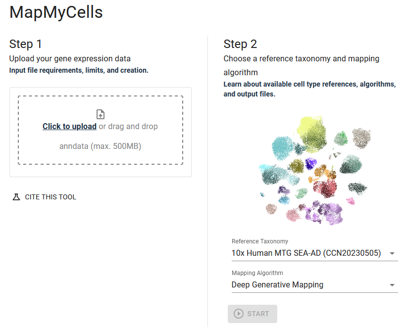
The steps to MapMyCells are as follows:

Go to (https://knowledge.brain-map.org/mapmycells/process/).
(Optional) Log in to MapMyCells.
Upload ‘Hodge2019.h5ad’ to the site via the file system or drag and drop (Step 1).
Choose “10x Human MTG SEA-AD (CCN20230505)” as the “Reference Taxonomy” (Step 2).
Choose the desired “Mapping Algorithm” (in this case “Deep Generative Mapping”).
Click “Start” and wait ~5 minutes. (Optional) You may have a panel on the left that says “Map Results” where you can also wait for your run to finish.
When the mapping is complete, you will have an option to download the “zip” file with mapping results. If your browser is preventing popups, search for small folder icon to the right URL address bar to enable downloads.
This download file (and the files therein) will have a long name. As of this writing the name is of the format (Upload file name)(Taxonomy name(id))(Mapping algorithm)(Unique run ID). Unzip this file, which will contain three or four files: “validation_log.txt”, “[long_name].json”, and “[long_name].csv”, and maybe [long_name]_summary_metadata.json. [long_name].csv contains the mapping results, which you need. The validation log will give you information about the the run itself and the json files will give you extra information about the mapping. You can ignore the latter files if the run completes successfully and if you are not a power user.
Copy [long_name].csv to your current working directory and rename it “Hodge2019_mapping.csv”).
You can now go back to R and continue the script below.

‍

5. Read mapping results into R

Let’s now look at the output results from the hierarchical clustering algorithm. We can read this into R using read.csv, but note that the first few lines contain metadata that need to be skipped, and begin with a ‘#’ character.

mapping <- read.csv("Hodge2019_mapping.csv",comment.char="#")
head(data.frame(mapping))

‍

In this taxonomy, MapMyCells maps input cells to the taxonomy at three increasing levels of resolution from coarsest class, to intermediate subclass, and finest supertype. In this human SEA-AD taxonomy there are 3 classes, 24 subclasses, and 139 supertypes.

The file consists of the following columns:

cell_id = the cell identifiers for your cells included in the initial h5ad files
class_label = the unique identifier for the best mapping class
class_name = the name of the best mapping class
class_softmax_probability = a score indicating the confidence that the cell mapped to the above class is accurately mapped (higher numbers are better, with 1 being the best; note that other mapping algorithms have different types of confidence scores with different names for this column)
and similar fields for subclass, supertype, and cluster. For finest level cluster there is an additional field

‍

6. Compare subclass and cluster assignments

As this data set is previously published, we already know the expected subclasses for each cell. Let’s check how well the mapped and clustered subclass calls match. Recall that we defined metadata as “annoIn” above. (This step will only work if your query data has previously assigned cell types, and may need slight modifications.)

comparison = table(mapping$subclass_name,annoIn$subclass)
heatmap(comparison, ylab = "Mapping", xlab = "Clustering",margins = c(10,10))

‍

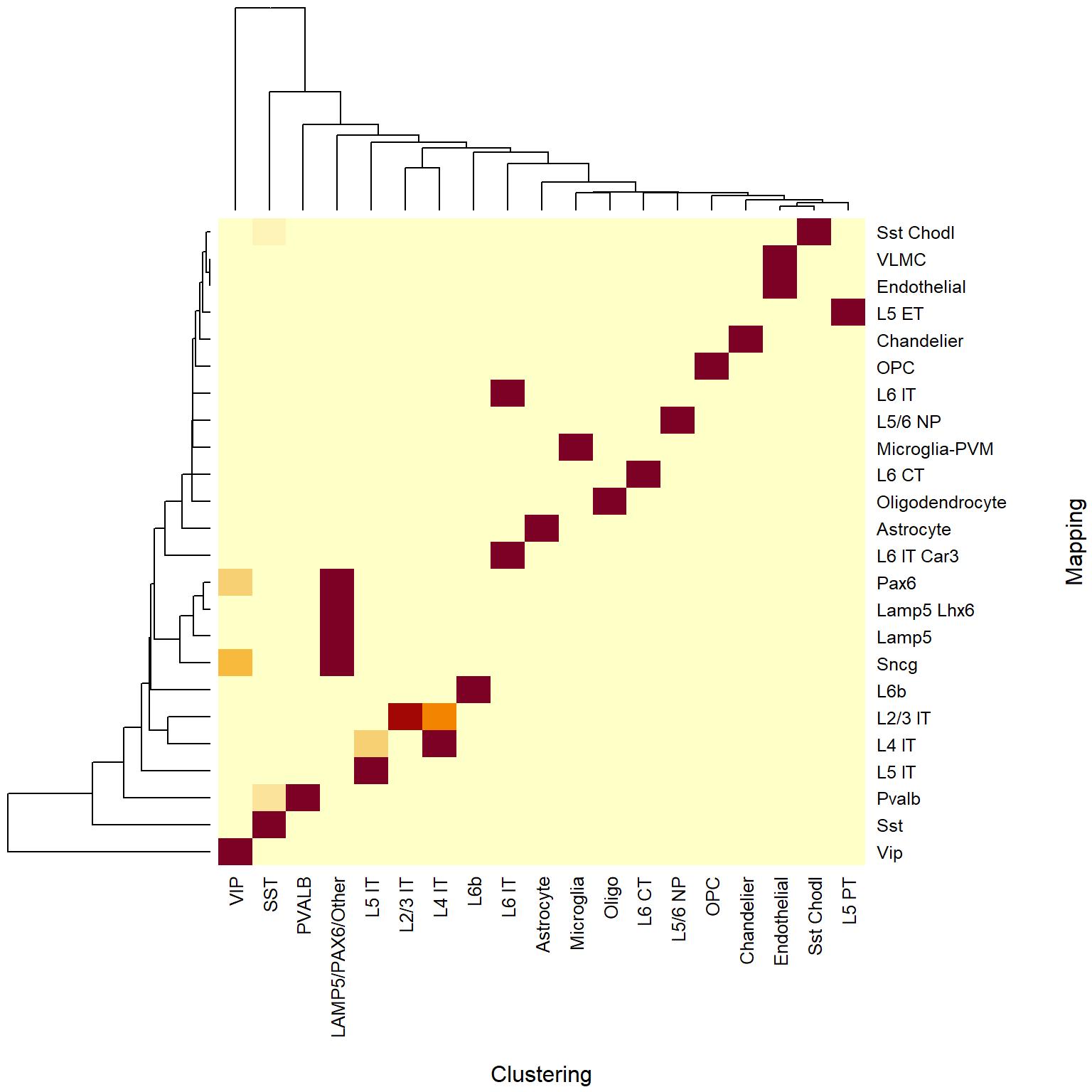
There is extremely good agreement, with most of the boxes showing all (red) or none (yellow) of the cells mapped to the same SEA-AD subclass coming from a given Hodge subclass call. (It turns out that the disagreements are largely due to differences in how subclasses are named or how their borders are defined between 2019 and 2023.)

Using the same strategy, we can see how clusters from Hodge et al 2019 correspond to supertypes from SEA-AD.

comparison = table(mapping$supertype_name,annoIn$cluster_label)
heatmap(comparison, ylab = "Mapping", xlab = "Clustering",margins = c(8,8), cexRow = 0.5, cexCol = 0.5)

‍

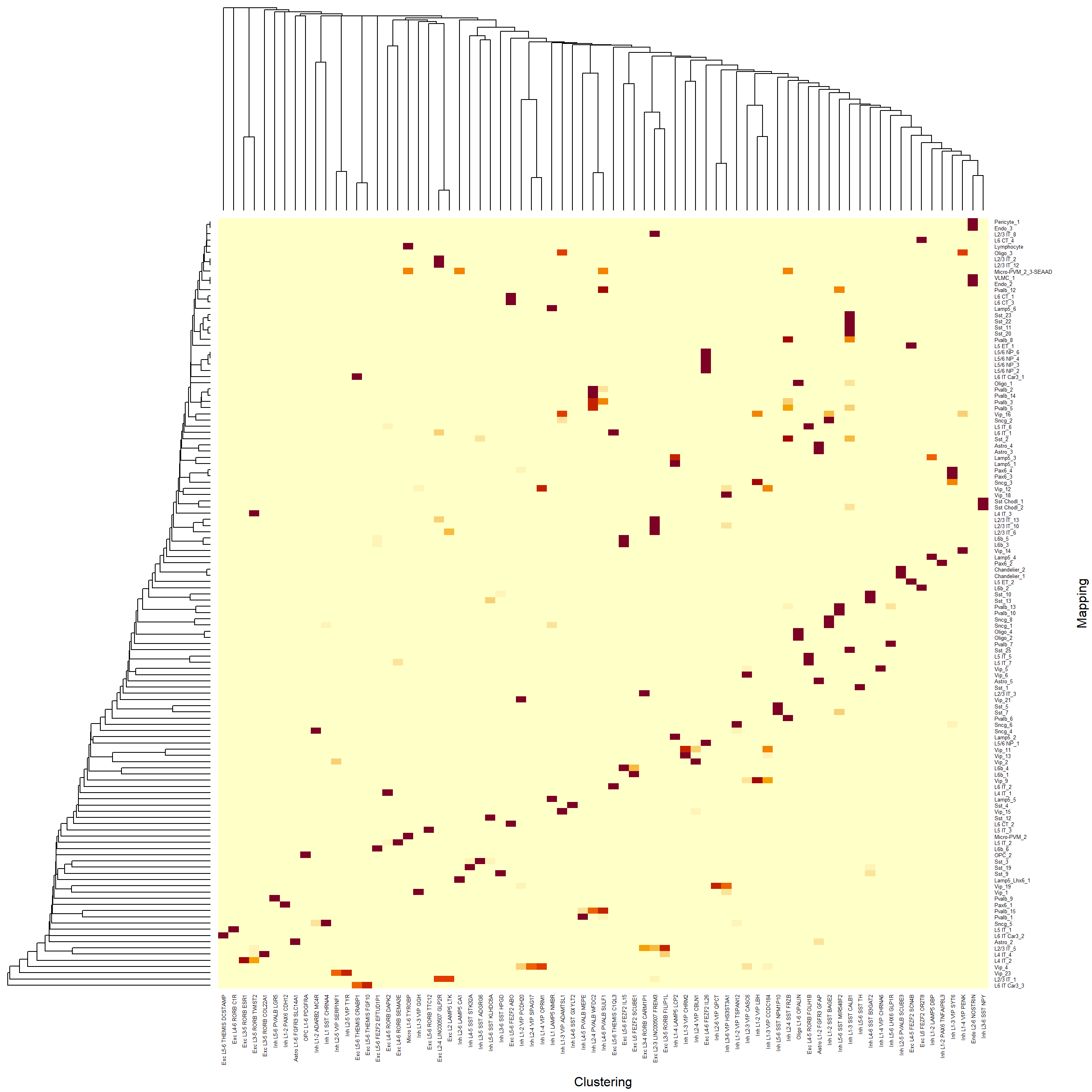
To do this properly would require more complicated analysis, but the main take-home here is that there is strong correspondence between initial cluster calls and mapping supertype assignments (lots of red and yellow, minimal intermediate colors).

‍

7. Visualize mapping results

# Since the query data corresponds to dataQC above, we will call it dataQC again
dataQC_h5ad <- read_h5ad('Hodge2019.h5ad')
dataQC <- t(as.matrix(dataQC_h5ad$X))
rownames(dataQC) <- rownames(dataQC_h5ad$var)
colnames(dataQC) <- rownames(dataQC_h5ad$obs)

‍

Now let’s visualize the mapping results. We will do this by saving the data in a Seurat object with mapping results as metadata, running the standard pipeline for creating a UMAP in Seurat, and then color-coding each cell.

# Create the Seurat object
dataSeurat <- CreateSeuratObject(counts = dataQC, meta.data = mapping)

# Standard Seurat pipeline
dataSeurat <- NormalizeData(dataSeurat, verbose = FALSE)
dataSeurat <- FindVariableFeatures(dataSeurat, verbose = FALSE)
dataSeurat <- ScaleData(dataSeurat, verbose = FALSE)
dataSeurat <- RunPCA(dataSeurat, verbose = FALSE)
dataSeurat <- RunUMAP(dataSeurat, dims = 1:10, verbose = FALSE)

‍

Now let’s make the plot for subclasses!

DimPlot(dataSeurat, reduction = "umap", group.by="subclass_name", label=TRUE) + NoLegend()

‍

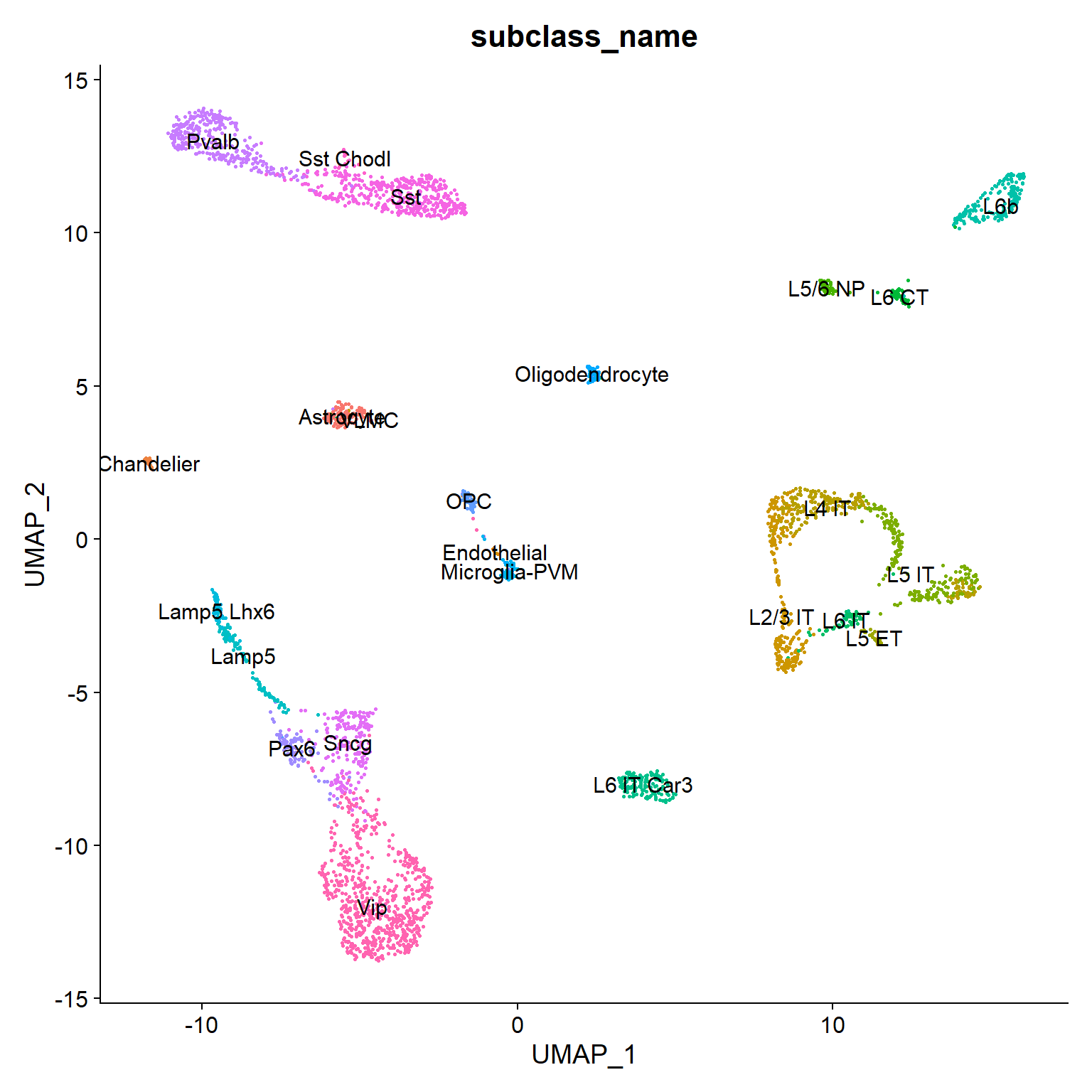
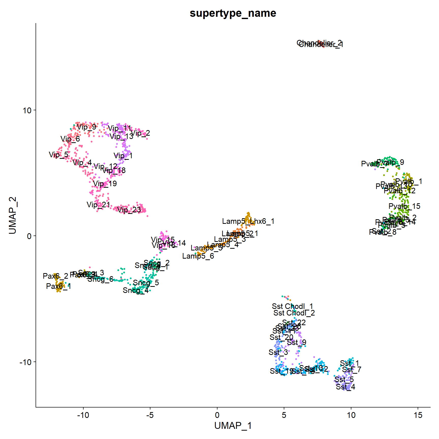
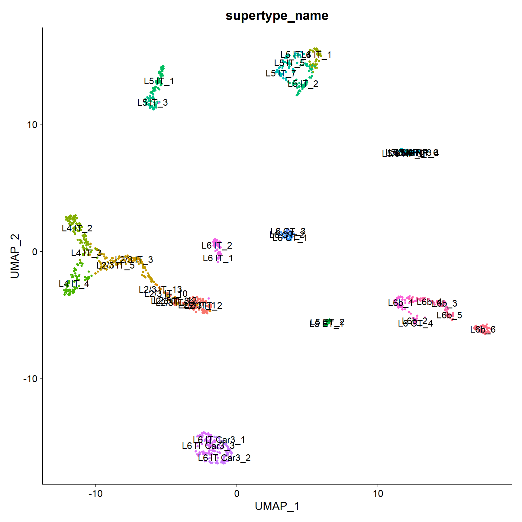
Here the data has not been clustered but rather the class assignments are assigned to the data in the UMAP. You can see that cells assigned different mapped types localize in different areas of the plot, suggesting that the label transfer works well. It’s worth noting that Seurat produces different UMAP configurations in different R environments, so your plot may not look exactly like this.

Now let’s repeat this analysis where we color-code UMAPs by supertype after separating cells mapped to different classes.

classes <- unique(mapping$class_name)
p       <- list()
for (cl in classes){
  datClass <- dataSeurat[,mapping$class_name==cl]
  datClass <- NormalizeData(datClass, verbose = FALSE)
  datClass <- FindVariableFeatures(datClass, verbose = FALSE)
  datClass <- ScaleData(datClass, verbose = FALSE)
  datClass <- RunPCA(datClass, verbose = FALSE)
  datClass <- RunUMAP(datClass, dims = 1:10, verbose = FALSE)
  p[[cl]]  <- DimPlot(datClass, reduction = "umap", group.by="supertype_name", label=TRUE) + NoLegend()
}
p[["Neuronal: GABAergic"]]

‍

p[["Neuronal: Glutamatergic"]]

‍

p[["Non-neuronal and Non-neural"]]

‍

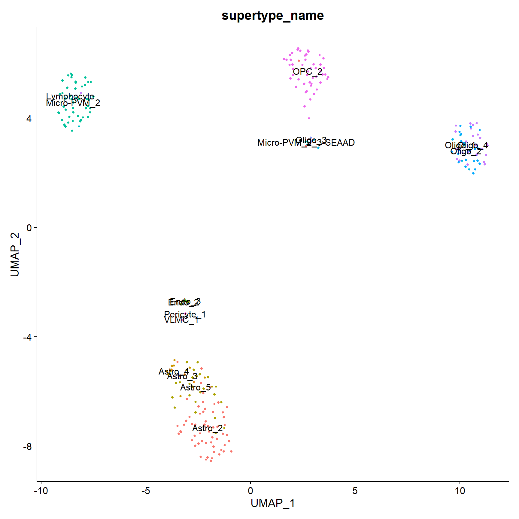
Once again, the supertypes shown largely segregate from one another without the need to apply clustering, suggesting this mapping works well even at higher resolutions. Scripts such as this can be used for visualizing and comparing mapping results. It’s worth noting that given how different these subclasses are from one another, viewing the data separately for each subclass or more carefully choosing variable genes would likely result in even better visualizations.

To output the session information we write the command, which is useful for reproducibility, especially for more complex scripts.

sessionInfo()## R version 4.2.2 (2022-10-31 ucrt)
## Platform: x86_64-w64-mingw32/x64 (64-bit)
## Running under: Windows 10 x64 (build 19045)
## 
## Matrix products: default
## 
## locale:
## [1] LC_COLLATE=English_United States.utf8 
## [2] LC_CTYPE=English_United States.utf8   
## [3] LC_MONETARY=English_United States.utf8
## [4] LC_NUMERIC=C                          
## [5] LC_TIME=English_United States.utf8    
## 
## attached base packages:
## [1] stats     graphics  grDevices utils     datasets  methods   base     
## 
## other attached packages:## [1] hodge2019data_1.0  anndata_0.7.5.6    SeuratObject_5.0.0 Seurat_4.4.0      
## 
## loaded via a namespace (and not attached):
##   [1] Rtsne_0.16             colorspace_2.1-0       deldir_1.0-9          
##   [4] ellipsis_0.3.2         ggridges_0.5.4         rstudioapi_0.15.0     
##   [7] spatstat.data_3.0-3    farver_2.1.1           leiden_0.4.3          
##  [10] listenv_0.9.0          ggrepel_0.9.4          fansi_1.0.5           
##  [13] codetools_0.2-19       splines_4.2.2          cachem_1.0.8          
##  [16] knitr_1.45             polyclip_1.10-6        spam_2.10-0           
##  [19] jsonlite_1.8.7         ica_1.0-3              cluster_2.1.4         
##  [22] png_0.1-8              uwot_0.1.16            shiny_1.7.5.1         
##  [25] sctransform_0.4.1      spatstat.sparse_3.0-3  compiler_4.2.2        
##  [28] httr_1.4.7             assertthat_0.2.1       Matrix_1.6-1.1        
##  [31] fastmap_1.1.1          lazyeval_0.2.2         cli_3.6.1             
##  [34] later_1.3.1            htmltools_0.5.6.1      tools_4.2.2           
##  [37] igraph_1.5.1           dotCall64_1.1-0        gtable_0.3.4          
##  [40] glue_1.6.2             RANN_2.6.1             reshape2_1.4.4        
##  [43] dplyr_1.1.3            Rcpp_1.0.11            scattermore_1.2       
##  [46] jquerylib_0.1.4        vctrs_0.6.4            nlme_3.1-163          
##  [49] spatstat.explore_3.2-5 progressr_0.14.0       lmtest_0.9-40         
##  [52] spatstat.random_3.2-1  xfun_0.40              stringr_1.5.0         
##  [55] globals_0.16.2         mime_0.12              miniUI_0.1.1.1        
##  [58] lifecycle_1.0.3        irlba_2.3.5.1          goftest_1.2-3         
##  [61] future_1.33.0          MASS_7.3-60            zoo_1.8-12            
##  [64] scales_1.2.1           promises_1.2.1         spatstat.utils_3.0-4  
##  [67] parallel_4.2.2         RColorBrewer_1.1-3     yaml_2.3.7            
##  [70] reticulate_1.34.0      pbapply_1.7-2          gridExtra_2.3         
##  [73] ggplot2_3.4.4          sass_0.4.7             stringi_1.7.12        
##  [76] highr_0.10             rlang_1.1.1            pkgconfig_2.0.3       
##  [79] matrixStats_1.0.0      evaluate_0.23          lattice_0.22-5        
##  [82] tensor_1.5             ROCR_1.0-11            purrr_1.0.2           
##  [85] labeling_0.4.3         patchwork_1.1.3        htmlwidgets_1.6.2     
##  [88] cowplot_1.1.1          tidyselect_1.2.0       parallelly_1.36.0     
##  [91] RcppAnnoy_0.0.21       plyr_1.8.9             magrittr_2.0.3        
##  [94] R6_2.5.1               generics_0.1.3         withr_2.5.2           
##  [97] pillar_1.9.0           fitdistrplus_1.1-11    survival_3.5-7        
## [100] abind_1.4-5            sp_2.1-1               tibble_3.2.1          
## [103] future.apply_1.11.0    KernSmooth_2.23-22     utf8_1.2.4            
## [106] spatstat.geom_3.2-7    plotly_4.10.3          rmarkdown_2.25        
## [109] grid_4.2.2             data.table_1.14.8      digest_0.6.33         
## [112] xtable_1.8-4           tidyr_1.3.0            httpuv_1.6.12         
## [115] munsell_0.5.0          viridisLite_0.4.2      bslib_0.5.1

Learn More

Onboarding

Step-by-step guide to using MapMyCells

Follow this complete guide to using MapMyCells. Learn data upload, cell mapping to taxonomies, result interpretation, and downloads.

While MapMyCells itself is straightforward (drag and drop!), there are a few steps before and after and some important tips and tricks to get the most out of the tool. This page goes through the steps from preparing your data for mapping to using the mapping results.

‍

Step 1: Preparing your data for mapping

MapMyCells requires a cell (rows) by gene (columns) matrix in an h5ad, csv, or csv.gz format as input. Gene identifiers are recommended, but gene symbols are also allowed. The green button walks through how to set up an input file, while the yellow buttons include start-to-finish R code for all steps of the process.

Input File Requirements & Conversion using R or Python | Start to finish: human middle temporal gyrus | Start to finish: mouse motor cortex

Frequently asked questions:

Can I map rat data to mouse brain cell types? While mapping between species is not officially supported, we have found that it works well for phylogenetically related species in some cases. Use GeneOrthology to convert gene symbols between species.

Can I use MapMyCells for bulk RNA-seq data? No. While MapMyCells will technically run with any sample by gene matrix, since each sample only gets a single cell type assignment and bulk tissue contains multiple cell types, these results will not be meaningful.

What should my h5ad file look like? The links above all provide the structure of h5ad files and links to examples. We also provide an example mouse h5ad file HERE.

I’ve never coded before. How do I make an h5ad file? We recognize this may be a challenge for some folks and plan to provide other options in the future. For now, we recommend Google Colaboratory which can run python code online with no setup needed.

‍

Step 2: Mapping your data to a reference

MapMyCells provides a variety of reference taxonomies and algorithms for mapping using both a web interface and code-based approaches, which all rely on the same file format. The blue buttons link to the mapping tools, while the green button describes the output files.

Go directly to the MapMyCells UI | Run the code on your own | Understanding algorithm output

‍Frequently asked questions:

I have too many cells to upload to MapMyCells. What should I do? The web interface requires cells <2GB in size. If your file is too big even after compression (see input links above) you have two options: (1) split your data set into multiple input files to upload separately, or (2) use the code version which does not have a size restriction. Since all algorithms treat each cell separately, you should get the same answer no matter how you divide your data set (although there might be very slight differences due to random sampling).

Can I map to only a subset of cell types in one of the reference taxonomies? Currently this is ONLY possible using code (some more details here). This functionality will be added to the web interface in 2025.

I’d like to create my own reference taxonomy to map against. How do I do that? While we encourage the use of reference cell type hosted on this site, we recognize this is not always possible. Scrattch.taxonomy provides both standard schema and associated file format for creation of cell type taxonomies in an h5ad format compatible with both R and python. You can also follow the approach from the previous question.

How should I decide which algorithm to use? In most cases, we recommend using the default. You could also consider trying multiple algorithms and comparing the results (see below). Regardless of the algorithm chosen, it is important to check that your mapping results make sense. More on this below.

Can I use other mapping algorithms? Currently three mapping algorithms are supported in MapMyCells. Additional approaches are available in scrattch.mapping (the companion package to scrattch.taxonomy). We also provide data for all taxonomies for download.

I’ve run MapMyCells and I can’t find my mapping results. What should I do? If your unpacked zip file does not have csv file with mapping results, check the validation log, which often will provide sensible messages explaining why your mapping failed. In most cases there is a problem with the input file. If you are still stuck, post a question to the Community Forum. Be sure to include your run ID, which looks something like this: “1698255812324-4d53ffc5-9c7c-4dff-b0b4-e4caf0923569”.

I’m struggling to understand how to use the python code. What should I do? The GitHub repository includes detailed documentation on recommended workflows, input formats, and outputs, including step-by-step Jupyter notebooks for defining and mapping against any taxonomy. If you are still stuck after reviewing these notebooks, post a question to the Community Forum.

‍

Step 3: Using mapping results

A common reason for running MapMyCells is to assign cell type names for user data that would replace or supplement the clustering analysis typically done as part of a single cell omics experiment. Therefore, a critical next step is to connect the cell type names and confidences returned from MapMyCells with original cell-level information in your study. The black button goes to an interactive tools to visualize and sanity check your mapping results after joining these data together, while the yellow buttons link to start-to-finish R scripts showing similar comparisons.

Interactive exploration: Annotation Comparison Explorer | Using R code: human middle temporal gyrus | Using R code: mouse motor cortex

Frequently asked questions:

Can I really forego clustering? In many cases, yes! If you are collecting cells from healthy mouse brain or from human neocortex in healthy or Alzheimer’s disease donors, our reference taxonomies will likely include all cell types in your sample. To improve cross-study comparison, we encourage using our cell types instead of defining your own.

How can I compare clustering and mapping results? Annotation Comparison Explorer (or ACE; above) provides interactive visualizations comparing any annotations. This includes confusion matrices and river plots comparing clustering and mapping results, and visualizations to explore individual clusters. When using ACE be sure to create a single csv file containing your mapping results, clustering, and any other relevant metadata. The R code examples provide additional code-based approaches for comparison.

I’ve successfully used MapMyCells. How can I cite your work? To cite the tool, please refer to MapMyCells as “MapMyCells (RRID:SCR_024672)” (see this link). We would also encourage users to cite the manuscript for the reference taxonomy.

‍

Getting help

The Allen Institute provides and ever-growing list of written (linked above) and video materials to aid users in successful use of MapMyCells. We also have an active Community Forum for reviewing previously asked questions and asking your own.

MapMyCells webinar (47 min) | Video tutorial (24 min) | Community Forum

‍

Learn More

Onboarding

Video

Cell Type Taxonomies Webinar Series

Join our webinar series on cell type taxonomies. Learn about brain cell classification from single-cell transcriptomics and taxonomy development.

The Cell Type Taxonomies A-Z: Webinar Series features presentations by Allen Institute scientists & staff for a full guide to brain cell types and taxonomies, and how and why to use these resources in your research. You can view them at the Allen Institute YouTube channel. To see upcoming iterations in this webinar series, visit https://alleninstitute.org/events/cell_type_az_webinars.

Check out some key webinars about brain-map and Brain Knowledge Platform resources:

Cell Types 101 | January 10, 2024

‍

What is a taxonomy? | January 31, 2024

‍

The techniques behind the Cell Type Knowledge Explorer | February 28, 2024

‍

Cross-species Cell Types | March 27, 2024

‍

What is your cell type: MapMyCells | April 24, 2024

‍

Introduction to ABC Atlas | May 22, 2024

Learn More

Video

Onboarding

Intro to the Adult Mouse Atlas

Get started with Allen Adult Mouse Atlas. Learn basic navigation, gene expression search, and how to explore mouse brain anatomy.

What is the Allen Mouse Common Coordinate Framework?

Allen Mouse Brain Common Coordinate Framework (CCFv3) is a 3D reference space by creating an average brain at 10um voxel resolution from serial two-photon tomography images of 1,675 young adult C57Bl6/J mice.

Using multimodal reference data, we parcellated the entire brain directly in 3D, labeling every voxel with a brain structure spanning 43 isocortical areas and their layers, 314 subcortical gray matter structures, 81 fiber tracts, and 8 ventricular structures.

The CCF is used in our informatics pipelines and online applications to analyze, visualize and integrate multimodal and multiscale data sets in 3D, and is openly accessible for research use under our Terms of Use.

Read this paper or documentation to learn more about the creation of the CCF.

‍

How do I view the Allen Mouse Common Coordinate Framework (CCF)?

There are two main ways to explore the CCF: in the 2D interactive atlas viewer or the online 3D Allen Brain Explorer.

‍

How do I download the CCF?

There are a couple of ways to download the average template volume, and annotation volume (volumes at 10, 25, 50, and 100 um isotropic resolution):

1. Using the AllenSDK

We recommend that you download atlas volumes using the AllenSDK, a Python package containing tools for accessing and using our data. Using the AllenSDK lets you easily download and organize the atlas and template volumes. Please see the example notebook for more information.

If you run into problems using the AllenSDK, let us know on the AllenSDK’s Github page.

2. Direct download from the server

We also make these volumes available through our download server. Read the overview and download instructions for more information.

‍

How do I download the labelled atlas images I see from the atlas image viewer?

An individual image can be downloaded directly from the atlas viewer via the menu on the top-right corner of the window.

See this post to learn how to access the images in bulk using the API or SDK.

‍

How do I download the structure ontology/tree?

The full structure ontology/tree can be downloaded from the API as a JSON, CSV or XML file.

Read this overview page for more information.

‍

How do I register my images to the CCF?

Image registration tools to align experimental data to the CCF is an active research area. Different modalities will likely required a targeted method to solve the problem.

List of community registration tools can be found in this post, the BICCN portal and NITRC.

‍

How do I access the registration code used in your pipeline?

The code in its current form it is highly coupled to the data modality, format and operations of the pipeline. It is likely the code will need to undergo major redevelopment for use in other contexts. For reference, the code is available on GitHub.

‍

How do I visualize CCF annotations on the original images?

Our typical workflow for analysis and display is to align image data from different specimens all into the CCF space for integrated analyses. Using the computed deformation field, it is possible to visualized CCF annotations of interest on the original images available through the AllenSDK. This GitHub repo has code and an example notebook to demonstrate this process step by step.

‍

How is the CCF being used by the neuroscience community?

We are keeping a list of publications and tools that uses the Allen Mouse CCF in this post. We invite others to add and contribute to the list.

‍

Related Resources

The Allen Mouse Brain Common Coordinate Framework: A 3D Reference Atlas - PubMed (nih.gov)

Community Forum - Allen Mouse CCF

Learn More

Onboarding

Video

Cell Type Knowledge Explorer video tutorial

Watch this video guide to Cell Type Knowledge Explorer. Learn to navigate single-cell data and explore cell type classifications and marker genes.

This video tutorial describes how to use the Cell Type Knowledge Explorer along with a bit about the data that went into the underlying cross-species, multimodal taxonomies in primary motor cortex. Need additional support? Please contact us!

BICAN presents: Cell Types Knowledge Explorer tutorial

Learn More

Video

No results. Please reduce your search parameters.

More Support Resources

Documentation

Reference atlases provide standard anatomical spaces across species and development

Explore

Citing Our Sources

Guidance on how to cite our resources when you use them in your work

Policy

Community Tools

Find community tools that utilize Allen Brain Map data

View Tools

Educator Resources

Support for teaching students with the Allen Brain Map

Explore

Have a specific question or need more help? Check out our Community Forum

Become part of a supportive community created by scientists for scientists. Find answer to your own questions and help your colleagues use brain-map resources to their full extend with Community Forum's diverse content.

Visit Community Forums

Tutorials & How-To's

Step 1: I open the BICAN Rapid Release specimen viewer and get a general overview by scrolling around.

Step 2: I use filters to reduce the list to only the grant that I’m interested in.

Step 3: I filter further by species & sex.

Step 4: I download the subset specimen metadata & file manifest and review them.

Step 5: I access the fastq files at NeMO archive

Manifest download and formatting

NeMO: Rapid Release Collections and Data Access

Introduction to Rapid Release Collection Types

Snapshot Collections (static)

Cumulative Collections (dynamic)

Rapid Release Collection (static)

Overview of Collection Types

Data Collections available through Rapid Releases

Accessing Rapid Release Data

Landing Pages

NeMO API endpoints

HTTPS location

Accessing NeMO Collections from Allen’s Brain Knowledge Platform (BKP)

NeMO Collections linked in BKP Project Pages

Metadata Search and File Manifest Retrieval from Specimen table of BKP’s Data Catalog

Step 1: I open the Genetic Tools Atlas and get a general overview by scrolling around.

Step 2: I use filters to reduce the list to only experiments that target the striatum.

Step 3: I filter further to a “finer labeled ROI” & cell type of interest.

Step 4: I review “Hall of Fame” entries and related image data

Step 5: I consider the enhancer suitable for my purposes and order it on Addgene - Vector ID lookup

Step 6: I explore non “Hall of Fame” entries and their image data

Step 7: I consider the enhancer suitable for my purposes and order it on Addgene - Addgene ID lookup

Overview

Using with the Whole Human Brain taxonomy

Using with the SEA-AD taxonomy

Using with the SEA-AD MERFISH data

YouTube Tutorial

YouTube Tutorials

Two-photon dataset tutorial

Neuropixels dataset tutorial

Downloading Atlas Images And Graphics

Structures And Ontologies

Image-to_Atlas

Prototype

Example

Parameters

Returns

Image-to_Image

Prototype

Example

Parameters

Returns

Image-to-Image 2-D

Prototype

Example

Parameters

Returns

Reference-To-Image

Prototype

Example

Parameters

Returns

Image-To-Reference

Prototype

Example

Parameters

Returns

Structure-To-Image

Prototype

Example

Parameters

Returns

Downloading 3-D Expression Grid Data

Prototype

Examples

Parameters

Response

Downloading 3-D Projection Grid Data

Prototype

Examples

Parameters

Response

YouTube Tutorial

Prototype