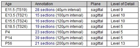
To provide a neuroanatomical framework for gene expression data, the Allen Developing Mouse Brain Reference Atlas was created with the expertise of Professor Luis Puelles, M.D., Ph.D. (University of Murcia, Spain). Sagittal full-color, high resolution web-based digital reference atlases have been created for seven stages of mouse brain development accompanied by a systematic developmental taxonomy of mouse brain structures.
The Allen Developing Mouse Brain Reference Atlases were designed to:
Allow users to directly compare gene expression patterns to an annotated developmental atlas;
Provide templates for the creation of 3-D computer models of the developing mouse brain;
Serve as a neuroanatomical foundation for informatics-based analysis tools.
In 2013, the reference atlas was updated to provide a deeper level of annotation. For more information on the reference atlas update and a description of the ontological levels, please refer to the Reference Atlas whitepaper located under the Documentation tab. Access to the previous reference datasets are available via links on the Reference Atlas landing page.
To access the reference atlas, you can click on one of the links from the landing page or you can select the key icon from the High Resolution Image Viewer to view the atlas in context with a gene expression experiment.
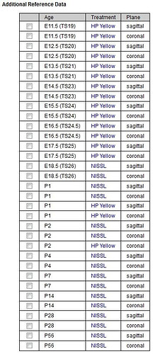
From the Reference Atlas landing page, you can also add reference data into your cart to enhance your exploration of gene expression data by clicking the checkboxes next to the desired reference dataset. Clicking “View Experiments” will allow you to view all selected datasets (including experimental data already present in the cart).
Translation Between the Adult and Developing Mouse Ontologies
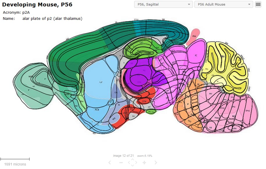
Given there are two structure ontologies for the mouse brain in the Allen Brain Atlas resources, we have created a way to overlay the Structure Ontology from Adult Mouse Atlas and the Developing Mouse Brain Atlas.
While in the “Developing Mouse Atlas, P56”, select “P56 Adult Mouse” atlas from the second drop-down menu and select “Outlines” from the Tools icon drop-down. This will show both Structure Ontologies overlayed together.
Reference Atlas Viewing with Gene Expression Data
Structure Ontology
The Structure Ontology for the Developing Mouse is listed hierarchically in the left-hand panel of the Interactive Atlas Viewer. By default the atlas is opened to level 3. Please see the Reference Atlas whitepaper available from the Documentation tab for more information on the Structure Ontology levels.
Each of the Developing Mouse atlases was drawn to a specific level and only those levels that were drawn will be available to navigate by clicking on the name. Those that are not available will be greyed out. Clicking on a structure name will take you to that drawn structure in the main image viewer.
Ontology Levels
Clicking on the ontology icon (see below) will open up the Developing Mouse Ontology defaulting at level 3.
Ontology Icon
The ontology levels in the Developing Mouse Atlas range from Level 00 (Neural Plate) up through higher differentiation levels to Level 13. Please see the Reference Atlas whitepaper available from the Documentation tab for a deeper explanation of the ontology levels. By clicking on the Ontology Levels (numbered squares above the ontology list) you will open the ontology to the level of detail indicated by the highlighted level.
Searching using the text box in the Ontology pane will allow you to browse through the ontology looking for specific regions. Using the “Sync” icon (see below), you can sync either image to its partner to view the gene expression in context with the reference atlas.
"Sync" Icon
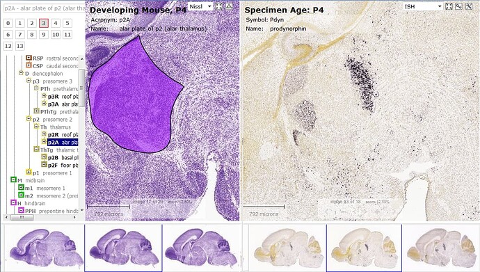
Given the difficulty of sectioning and programatically aligning these small specimen, you have the option of viewing a reference dataset with each gene expression specimen that will also outline a small structure of interest. To do this, choose the reference atlas from the Atlas dropdown menu (either Feulgen-HP or Nissl, depending upon the age) and select on the reference data set to outline your desired structure.
In the below image, gene expression is located in a region of the prethalamus.
Allen Developing Mouse Brain Atlas: Brain Explorer® 3D Viewer
Master Allen Brain Explorer desktop application for 3D visualization. Navigate brain atlases, view gene expression, and create custom visualizations.
Brain Explorer® 3D Viewer is an application for viewing brain anatomy and gene expression data in three dimensions in the framework of the Allen Developing Mouse Brain Reference Atlas.
Using Brain Explorer, you can:
View fully interactive versions of the Allen Developing Mouse Reference Atlases in 3-D.
View gene expression data in 3-D at 200 µm 3 resolution.
View expression data from multiple genes superimposed on each other in 3-D.
Navigate the high-resolution 2-D ISH images using the 3-D model.
Link to associated gene metadata on the Allen Developing Mouse Brain Atlas web application.
Installation
Windows
Systems requirement: minimum configuration
Operating System: Microsoft Windows 7
CPU: Intel Core Duo or AMD 1.8GHz
System Memory: 1GB
Graphics Card: Hardware 3D OpenGL accelerated AGP or PCI Express with 64MB RAM
Screen: 1024x768, 32-bit true color
Hard Disk: 200MB free space
Note: Brain Explorer is known to work with the following video chipsets: nVidia GeForce 9400/9600, nVidia Quadro FX 1800/3800/5600, AMD Radeon 9600, AMD Radeon HD 3200/4550, Intel Q35/Q45 Express.
For the best performance, please check with your video card vendor for the latest available drivers before using Brain Explorer. The Windows version of the Brain Explorer viewer is available here. Double-click the downloaded BrainExplorer2.msi file and follow the prompts.
Mac
Systems requirement: minimum configuration
Operating System: OS X 10.6.8
CPU: Intel 1.8GHz
System Memory: 1GB
Graphics Card: 3D-capable with 64MB RAM
Screen: 1024x768, 32-bit millions of colors
Hard Disk: 200MB free space
Note: Please install the latest system updates from Apple to ensure you have the latest video card drivers.
The Mac version of the Brain Explorer viewer is available here. Double-click the downloaded zip file to unpack Brain Explorer.
Installing Atlases
A one-time download containing anatomy files is needed following installation of the Brain Explorer application. The first time you open the Brain Explorer software, you will be asked to choose to download files for the Allen Mouse and Allen Human Brain atlases. Click on the atlases you would like to use and then click the Install button.
To download missing atlases on the PC, go to the Help menu and select Download Atlases. On the Mac, the command is in the Brain Explorer 2 menu.
Getting Updates
The Brain Explorer application will inform you when updates to the Brain Explorer application itself or its atlases are available. New data may not be available for viewing until you install the required updates.
Viewing Gene Expression
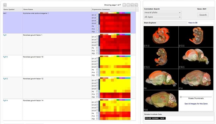
To load gene expression data into the Brain Explorer viewer: go to the Allen Developing Mouse Brain Atlas and perform a search. Your search brings back a list of genes that fit your search criteria. Click on a gene name to select a gene of interest. 3-D thumbnails at all developmental stages of the gene expression pattern from that gene will load to the right. Click on the blue “View in 3D” link to launch the Brain Explorer application and load each experiment.
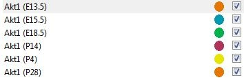
The Image Viewer will display the gene expression representations in 3-D for your gene of interest across all stages. Each stage will default to separate color schemes for each developing stage. For each developing stage, a sphere represents expression re-sampled to a grid resolution that is dependent on the stage in question (see the Informatics Data Processing whitepaper available in the Documentation. Larger spheres correspond to a greater density of expression in that voxel.
You can filter the developmental stages by hovering your mouse over the age to bring up an “X” or a magnifying glass. Clicking on the “X” will close that experiment, clicking on the magnifying glass will remove all the other stages from the viewer.
You can select a sphere by clicking on it. Spheres can be deselected by clicking on blank space. The original ISH image of the selected sphere will be displayed blended with the expression heat mask in the lower left-hand portion of the screen. The blending can be adjusted by selecting Image Controls from the View menu and moving the Image Blending slider. Clicking on the arrow in the top right-hand corner of the zoomed ISH image will open the corresponding ISH image in a high resolution image viewer.
The information at the upper-left corner of the main Brain Explorer window summarizes the expression detected in the selected grid location. These numbers include the average expression density and intensity (over pixels). The Informatics Data Processing White Paper describes how the measurements were obtained.
To change the gene expression representation, click on the “Data” menu and select an option under “Raw” colors.
A compass in the right-hand corner of the Image Viewer can be used to rotate the brain(s) by clicking and dragging your cursor. You can zoom using either the wheel on your mouse or using the Zoom scrollbar in the lower right-hand corner of the Image Viewer.
Expression Thresholds
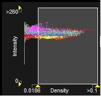
A way to control expression visibility is by setting thresholds on expression values. This method can restrict visible spheres to different combinations such as low intensity and low density or high intensity and low density.
The graph in the lower right-hand corner shows a dot for each data point (sphere) in a gene expression file, and the color of the dot corresponds to the anatomic annotation in the same way the atlas colors display mode works. Each data point is plotted according to its density on the x-axis and its intensity on the y-axis.
The color scale on the left-hand side of the graph corresponds to the expression level heat map used to color the spheres, color coded to the reference atlas structures. The numbers along each axis show the values at the yellow triangles.
The thresholds can be changed by resizing the white box. Any edge or corner of the box can be clicked and dragged to re-size it. You can also click and drag in the center of the box to move the box.
Structure Ontology Viewer
The Structure Ontology Viewer shows the entire collapsible ontology for the developing mouse brain as defined by the Allen Developing Mouse Reference Atlas. The first column represents the color of the reference atlas for that structure. The two columns to the right determine the type of data displayed in the Image Viewer. “A” represents atlas structure and when checked, will show a visual representation of that structure in the Image Viewer. “D” represents gene expression and when checked, will show gene expression in that structural domain.
The default organization for the Structure Ontology is the Hierarchical View, but if you are unfamiliar with the ontology, you can click on the Alphabetical View to see the structure list in alphabetical order.
The Bookmarks tab is a space where you can create and save favorite views of the brain. Several default views are already saved that will rotate the brain back into common viewing frames.
Gene List
This section displays the experiments you have selected and downloaded in this session. Right clicking on the gene name will bring up a menu where you can, 1) view the gene detail page (Get Info), 2) be taken to a zoomed in image from this experiment (View Images), 3) copy meta information to the clipboard, such as symbol, name, Entrez ID, image-series ID (Copy Info), 4) activate a Correlation search by finding experiments with similar expression profiles (Find Similar) or 5) close the experiment and remove it from the list and the 3-D view (Close).
Gene Search
To search for genes within the Brain Explorer application, go to the Search box located above the ontology panel and type in the gene symbol or part of a gene name.
The list of results shows gene name, gene symbol along with a 3-D summary thumbnail of the expression for each experiment matching the search. The expression thumbnail represents a maximum expression projection rendering: the denser the expression in a region the more “solid” the appearance. Reference atlas colors are additionally layered on top.
To load an experiment for viewing, click on the “Download” button under the gene name.
Toolbar
Button
Operation
Selects cursor rotation tool mode
Selects cursor pan tool mode
Selects cursor selection tool mode
Toggle Sagittal Atlas section viewing
Toggle Coronal Atlas section viewing
Toggle Horizontal Atlas section viewing
Centers the Viewer on the current pinpointed expression data point
Turns on the cutting planes
Toggles the Structure Ontology and Gene List View
Advanced Features
Atlas Menu:
You can show opaque three dimensional structures of the brain by “showing” or “hiding” structures from this menu. The “Transparent” function allows you to see transparent views of the structures to view the anatomical relationships between them.
Selecting the sagittal, coronal or horizontal sections (or clicking on one of the section image buttons in the toolbar) will superimpose a single plane of the reference images (Nissl or Feulgen-HP) from each brain on your image space. These planes can be moved once the selection tool mode button in the toolbar is selected. Selecting “Show Annotation on Section” from this menu will color the reference images according to the brain structure ontology.
Data Menu:
When you have a gene selected, the Data menu allows you to show all expression, hide all expression (for instance to then select a single structure) or toggle expression (for instance, unselect your region of interest then toggle to see expression in only that region).
You can also show or remove threshold controls and choose the visual representation of your data from this menu. There are several options under “Raw” colors:
User defined: Each experiment is rendered in user specified color. This mode is useful to distinguish between individual experiments when multiple experiments are being displayed.
Atlas: In this mode the sphere is colored by the corresponding reference atlas structure color. This mode is useful for quickly seeing the annotated regions where a gene is expressing.
Signal Level: This mode displays average expression intensity and is useful for identifying areas of very high expression.
Jet: Applies the common “jet” colormap to the data.
To be taken to the experimental detail page, select “Get Info”. To see a high resolution image view of this experiment, choose “View Images”. These functions are also available by right-clicking on the gene name in the Gene List.
Choose “Find Similar” to find similar genes to the selected experiment. This uses the same Correlation Search functionality as in the web application.
Clipping Planes:
When this function is selected, either by toggling the cutting tools button in the toolbar or selecting “Clipping Planes” from the View drop down menu, you can make coronal, sagittal or horizontal cuts in your view of the brain and related data. To cut in a particular plane, make sure the cursor is in selection tool mode, and then click and drag on the plane you are interested in clipping.
Troubleshooting
Windows
Graphics
If you are using a desktop computer, you should obtain drivers from the video card manufacturer. First, identify the video card. Go the Start menu and open the Control Panel. Open the Display control panel and go to the Settings tab. Click the Advanced button and go to the Adapter tab. Your video card vendor and model name will be displayed at the top of the window under Adapter Type. Please go to the manufacturer’s web site, locate the driver download, and follow the instructions on the website or included with the downloaded file.
If you are using a laptop computer, you will need to go to your laptop manufacturer’s web site to locate the latest video drivers.
You can also activate an alternate drawing mode in Brain Explorer. Go to the View menu and select Options. Check the Draw faster but at lower quality button and uncheck the Synchronize drawing with the monitor’s vertical refresh button. Set the Multisample setting to Off.
If you are using multiple video cards from different vendors, the 3-D display may not work correctly on all attached monitors.
Uninstalling
Use the Add/Remove Programs control panel or the uninstall link in the Brain Explorer folder in the Start menu. Additional data that are not automatically uninstalled are located at the following locations:
Windows XP
Atlas data: C:\Documents and Settings\userid\Local Settings\Application Data\Allen Institute\Brain Explorer 2 User settings: C:\Documents and Settings\userid\Application Data\Allen Institute\Brain Explorer 2
Windows Vista and Windows 7
Atlas data: C:\Users\userid\AppData\Local\Allen Institute\Brain Explorer 2 User settings: C:\Users\userid\AppData\Roaming\Allen Institute\Brain Explorer 2
Proxy Settings
If you use a proxy server, the Brain Explorer application will use the proxy settings from the Internet Options control panel in the Windows Start menu. Please refer to the Windows documentation for help on proxy settings.
Mac
Uninstalling
Drag the Brain Explorer 2 icon to the trash. The Brain Explorer application generates the following files, which can also be dragged to the trash.
If the Brain Explorer application is not running smoothly, first try to free up as much memory as possible by quitting all other open applications. You can also activate an alternate drawing mode. Go to the Brain Explorer 2 menu and select Preferences. Check the Draw faster but at lower quality button and uncheck the Synchronize drawing with the monitor’s vertical refresh button. Set Multisampling to Off.
Learn about API For Allen Developing Mouse Brain Atlas with comprehensive guides and examples from Allen Institute for Brain Science.
The Allen Developing Mouse Brain Atlas provides in situ hybridization (ISH) image data for approximately 2,000 genes over embryonic and postnatal timepoints. Each data set is processed through an informatics analysis pipeline to obtain spatially mapped quantified expression information.
From the API, you can:
Download images
Download quantified expression values by structure
Download quantified expression values as 3-D grids
Query the correlative search service
Query the image synchronization service
Download atlas images, drawings and structure ontology
This document provides a brief overview of the data, database organization and example queries. API database object names are in camel case. See the main API documentation for more information on data models and query syntax.
Experimental Overview and Metadata
Experimental data from this atlas is associated with the “Developing Mouse Brain” Product.
Multiple genes were assayed using each Specimen. Typically, the sectioning scheme divided each brain into 4 to 8 interleaving SectionDataSets depending on the age of the specimen.
Section thickness is 20 micron for the earlier timepoints up to P4 and 25 micron for P14 and older. Section thickness is an attribute of the SectionDataSet object.
Image resolution is variable (0.99 - 1.049 microns) and is reported as an attribute of SectionImage.
Each gene was assayed with one sagittal SectionDataSet at each of the 7 main developmental timepoints (E11.5, E13.5, E15.5, E18.5, P4, P14, P28). A subset of genes also has coronal SectionDataSets, replicate sagittal experiments and/or data for intermediate and aging timepoints.
To support the generation of structure/age summaries for the web application, one sagittal SectionDataSet is selected as the representative for each age. This is reported as the boolean delegate attribute of SectionDataSet.
From the API, detailed information about Genes, Probes, SectionDataSets and SectionImages can be obtained using RMA queries.
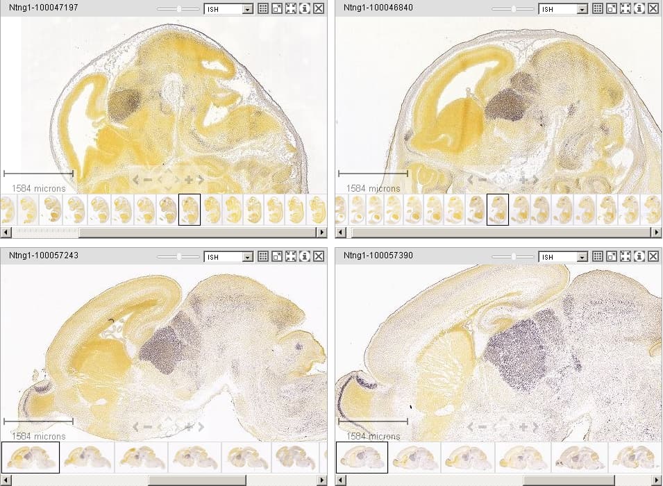
Figure: There are 11 SectionDataSets associated with gene netrin G1 (Ntng1). Screenshot shows SectionDataSets for timepoints E13.5, E15.5, E18.5 and P4.
See the image download page to learn how to download images at different resolutions and regions of interest.
Informatics Data Processing
The informatics data processing pipeline produces results that enable the navigation, analysis and visualization. The pipeline consists of the following components:
a set of age-matched annotated 3-D reference spaces,
an alignment module,
an expression detection module,
an expression gridding module, and
a structure unionizer module.
The output of the pipeline is quantified expression values at a grid voxel level and at a structure level according to the integrated reference atlas ontology. The grid level data are used downstream to provide a correlative gene search service and to support visualization of spatial relationships. See the informatics processing whitepaper for more details.
3-D Reference Models
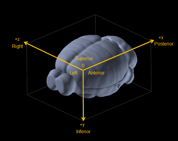
The backbone of the automated pipeline is a set of annotated 3-D reference spaces for each of the 7 developmental stages. For each stage, a brain volume was reconstructed from section images from a single specimen. Each 3-D reference space is in PIR orientation (+x = posterior, +y = inferior, +z = right).
Figure: All references spaces are in PIR orientation where x axis = Anterior-to-Posterior, y axis = Superior-to-Inferior and z axis = Left-to-Right.
Structural delineation were extracted from the associated 2-D reference atlas plates and interpolated to create 3-D annotations. Structures in the reference atlas are arranged in a hierarchical organization. Each structure has one parent and denotes a “part-of” relationship. Structures are assigned a color to visually emphasize their hierarchical positions in the brain. Note: the structural hierarchy used in this atlas is based on a systematic developmental ontology that differs from the ontology used for processing the Allen Mouse Brain Atlas.
Three volumetric data files are available for download for each reference space from our download server:
atlasVolume: uchar (8bit) grayscale Nissl or Feulgen-HP yellow volume of the reconstructed brain.
annotation: uint (32bit) structural annotation volume matching the atlasVolume. The value represents the ID of the finest level structure annotated for the voxel. Note: the 3-D mask for any structure is composed of all voxels annotated for that structure and all of its descendents in the structure hierarchy.
gridAnnotation: uint (32bit) structural annotation volume at grid resolution.
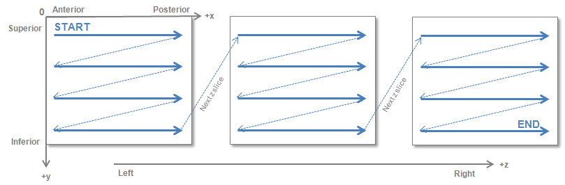
All volumetric data is stored in an uncompressed format with a simple text header file in MetaImage format. The raw numerical data is stored as a 1-D array as shown in the figure below.
Figure: Packing of 3-D volumetric data into a 1-D numerical array.
The atlas volumedimension and resolution for each ReferenceSpace vary with age, scanning platform and gene sampling density as listed in the table below.
Example Matlab code snippet to read in the P4 atlas and annotation volume:
% ------------
% Download and unzip the P4(ReferenceSpace=6) atlasVolume and annotation zip files
% ------------
% atlas volume size
size = [724,403,398];
% VOL = 3-D matrix of atlas Nissl volume
fid = fopen('P4_atlasVolume/atlasVolume.raw', 'r', 'l' );
VOL = fread( fid, prod(size), 'uint8' );
fclose( fid );
VOL = reshape(VOL,size);
% ANO = 3-D matrix of annotation labels
fid = fopen('P4_DevMouse2012_annotation/annotation.raw', 'r', 'l' );
ANO = fread( fid, prod(size), 'uint32' );
fclose( fid );
ANO = reshape(ANO,size);
% Display one coronal section
figure;imagesc(squeeze(VOL(362,:,:)));colormap(gray);
figure;imagesc(squeeze(ANO(362,:,:)));colormap(lines);
% Display one sagittal section
figure;imagesc(squeeze(ANO(:,:,115)));colormap(lines);
figure;imagesc(squeeze(VOL(:,:,115)));colormap(gray);
Example Matlab code snippet to read in the P4 grid annotation volume:
% -----------% Download and unzip the P4 (ReferenceSpace=6) gridAnnotation zip files
% -----------% grid volume size
sizeGrid = [77,43,50];
% ANOGD = 3-D matrix of grid-level annotation labels
fid = fopen( 'P4_DevMouse2012_gridAnnotation/gridAnnotation.raw', 'r', 'l' );
ANOGD = fread( fid, prod(sizeGrid), 'uint32' );
fclose( fid );
ANOGD = reshape(ANOGD,sizeGrid);
% Display one coronal and one sagittal section
figure;imagesc(squeeze(ANOGD(36,:,:)));colormap(lines);
figure;imagesc(squeeze(ANOGD(:,:,14)));colormap(lines);
Image Alignment
The aim of image alignment is to establish a mapping from each SectionDataSet to its exact or closest age matched ReferenceSpace. The reference-space-id attribute indicates which reference space the data has been aligned to. The module reconstructs a 3-D Specimen volume from its constituent SectionImages and registers the volume to the 3-D reference model by maximizing image correlation.
Once registration is achieved, information from the 3-D reference model can be transferred to the reconstructed Specimen and vice versa. The resulting transform information is stored in the database. Each SectionImage has an Alignment2d object that represents the 2-D affine transform between an image pixel position and a location in the Specimen volume. Each SectionDataSet has an Alignment3d object that represents the 3-D affine transform between a location in the Specimen volume and a point in the 3-D reference model. Spatial correspondence between any two SectionDataSets from different Specimens can be established by composing these transforms.
For convenience, a set of “Image Synchronization” API methods is available to find a corresponding position between SectionDataSets, the 3-D reference model and structures. Note that all locations on SectionImages are reported in pixel coordinates and all locations in 3-D ReferenceSpaces are reported in microns. These methods are used by the Web application to provide the image synchronization feature in the multiple image viewer.
To support image synchronization across reference spaces, each space has been co-registered and scaled to every other space using a 12 parameter affine transform, allowing brains of different ages to be roughly compared. The image synchronization API methods automatically perform the cross-space transform when requesting to sync data from different reference spaces.
[type or paste code here](http://api.brain-map.org/api/v2/image_to_atlas/101121829.json?x=5752&y=3312&atlas_id=181276165)
Figure: Cross timepoint image synchronization on the Web application. Multiple SectionDataSets in the Zoom-and-Pan (Zap) viewer can be synchronized to the same approximate location across different ages. Screenshot taken after synchronization of 5 other Ntng1 SectionDataSets at E13.5, E15.5, E18.5, P14 and P28 to the P4 (lower-left) SectionDataSet.
Figure: Screenshot taken after synchronization of the E11.5, E13.5, E15.5, P4, P14 and P56 atlases to the P4 ISH SectionDataSet (lower-left in the previous figure).
Expression Detection
For every ISH SectionImage, a grayscale mask is generated that identifies pixels corresponding to gene expression. The detection algorithm is based on adaptive thresholding and mathematical morphology.
The expression mask image is the same size and pixel resolution as the primary ISH image and can be downloaded through the image download service.
Expression Gridding
For each SectionDataSet, the Gridding module creates a low resolution 3-D summary of the gene expression and projects the data to its exact or closest age matched ReferenceSpace. Casting all data into a canonical space allows for easy cross-comparison of gene expression data within each stage. The expression data grids can also be viewed directly as 3-D volumes or used for analysis such as correlative searches.
Each image in a SectionDataSet is divided into a grid resolution squares. Grid resolution varies with age ranging from 80 x 80 µm at E11.5 to 200 x 200 µm at P28. Pixel-based gene expression statistics are computed using information from the primary ISH and the expression mask:
expression density = sum of expressing pixels / sum of all pixels in division
expression intensity = sum of expressing pixel intensity / sum of expressing pixels
expression energy = expression intensity * expression density
Each per-image 2-D expression grid is smoothed and rotated to form a 3-D grid. Z-direction smoothing is applied to the 3-D grid which is then transformed into the targeted reference space.
Grid data can be downloaded for each SectionDataSet using the 3-D Expression Grid Data Service. The service returns a zip file containing the volumetric data for expression density, intensity and/or energy in an uncompressed format with a simple text header file in MetaImage format. Structural annotation for each grid voxel can be obtained via the ReferenceSpace gridAnnotation volume file.
Note: Coronal SectionDataSets span both hemispheres while sagittal SectionDataSets only span the left hemisphere. Voxels with no data are assigned a value of “-1”.
The expression data grid can be viewed in the Brain Explorer® 2 desktop program. Each grid voxel is rendered as a colorized sphere where the diameter represents expression energy and the color encodes expression intensity. In addition, a preview of the expression data grid is shown on the Web application as a series of maximum density projection images.
Example Matlab code snippet to read an energy grid volume:
%------------% Download and unzip the energy grid file for P4 Rora Pdyn SectionDataSet
%-----------% grid volume size
sizeGrid = [77,43,50];
% ENERGY =3-D matrix of expression energy grid volume
fid = fopen('Rora_P4_sagittal_100054927/energy.raw', 'r', 'l' );
ENERGY = fread( fid, prod(sizeGrid), 'float' );
fclose( fid );
ENERGY = reshape(ENERGY,sizeGrid);
% Display one coronal andone sagittal section
figure;imagesc(squeeze(ENERGY(36,:,:)));colormap(gray);
figure;imagesc(squeeze(ENERGY(:,:,14)));colormap(gray);
Structure Unionization
Expression statistics at a structural level are also computed by combining/unionizing grid voxels with the same 3-D structural label. Expression statistics are encapsulated as a StructureUnionize object associated with one Structure and one SectionDataSet. StructureUnionize data is used in the web application to display expression summary colormaps for a set of coarse structures over development.
Expression statistics are encapsulated as a StructureUnionize object associated with one Structure and one SectionDataSet and can be downloaded via RMA.
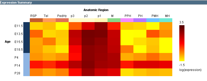
StructureUnionize data is used in the web application to generate an expression summary heatmap for a set of coarse structures over the 7 main developmental timepoints assayed.
Example:
Fetch expression energy values for the delegate SectionDataSet at each of the 7 developmental ages for coarse-level structures RSP, Tel, PedHy, p3, p2, p1, M, PPH, PH, PMH and MH in CSV format
Figure: Gene expression “heatmap” from the gene detail page of Tcf7l2 for 11 gross anatomical regions over 7 developmental timepoints.
Expression Grid Search Service
A expression grid service has been implemented to allow users to instantly perform a correlation search over the ~2,000 genes to find genes that have a similar spatio-temporal profile to a seed gene.
The expression grid search service is available through both the Web application and API.
To perform a Correlation search, a user selects a seed Gene, a spatial domain and a set of timepoints over which the similarity comparison is to be made. All voxels belonging to any of the domain structures and specified timepoints form the domain voxel set. Pearson’s correlation coefficient is computed between the domain voxel set from the seed Gene and every other Gene in the Product. The return list is sorted by descending correlation coefficient.
Note: Only the 7 main developmental timepoints (E11.5, E13.5, E15.5, E18.5, P4, P14, P28) can be used as temporal domain. For each timepoint, the delegate SectionDataSet is used in the computation.
See the connected service page for definitions of service::dev_mouse_correlation parameters.
Example:
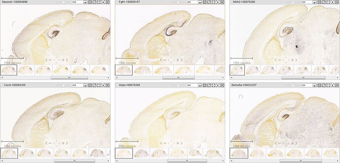
Correlation search for genes with similar expression to Neurod1 within the telencephalic vesicle (Tel) at age P4
Figure: Screenshot of top returns of a correlation search for genes with similar expression as Neurod1 within the telencephalic telencephalic vesicle at age P4.
Example:
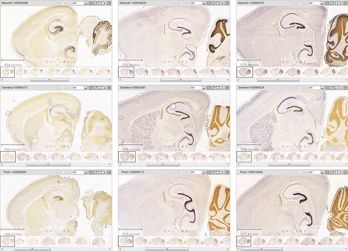
Correlation search for genes with similar expression to Neurod1 within Tel over multiple ages P4, P14, P28
Figure: Screenshot of the top 2 returns (Sowaha, Prox1) of a correlation search for genes with similar expression as Neurod1 within the telencephalic vesicle at ages (left to right) P4, P14, P28.
Example:
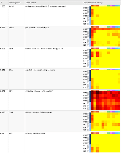
Correlation search for genes with similar expression to Nr5a1 over the whole neural plate (NP) and across all 7 ages
Figure: Screenshot of the top returns of a correlation search for genes with similar expression as Nr5a1 over the whole neural plate (NP) and across all 7 ages. Each gene is represented by an expression “heatmap” for 11 gross regions.
Expert Manual Annotation
ISH data for ages E11.5, E13.5, E15.5 and E18.5 were manually annotated to provide accurate gene expression characteristics for fine level structures. For each SectionDataSet and Structure, gene expression is scored with intensity (Undetected, Low, Medium, High), density (Undetected, Low, Medium, High) and pattern (Undetected, Full, Regional, Gradient) attributes.
Manual annotation results can be accessed through RMA and can be used to search data.
Note: the structural hierarchy associated with the manual annotation differs from the Ontology used for informatics processing of the ISH data.
Examples:
Download manual annotation for gene Tcf7l2 at E11.5
Learn about Developmental Anatomic Gene Expression Atlas AGEA with comprehensive guides and examples from Allen Institute for Brain Science.
AGEA is an interactive relational atlas based on spatial correlations of gene expression data for ~2000 genes in the Allen Developing Mouse Brain Atlas.
AGEA for the Developing Mouse Brain is used to understand how voxels of the brain are related by gene expression (Correlation), and to find genes expressed at a particular voxel (Gene Finder). Click on the AGEA tab to get started.
Correlation Mode
In correlation mode, use the seed selector to select a starting age by clicking on your age of interest. The next three columns will show you the age you selected flanked by the nearest developmental ages. Also shown in the column headers are the structure and location of the selected voxel and the Pearson’s correlations (please see Informatics whitepaper available from the Documentation tab).
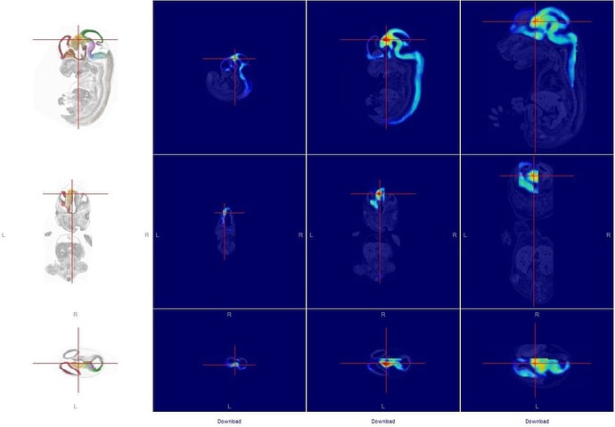
Select a “seed” voxel using the cross hairs in the left hand column from one of the planes of view. The three columns to the right show correlation maps of how other voxels are related to the seed voxel based upon the gene expression of approximately 2000 genes.
Seed Selector
To begin, select an age from the upper left hand corner. Maps of the age-appropriate reference space are shown in sagittal, coronal and horizontal planes in the left-most column. Navigate by clicking on a spot in one plane of view; this will appropriately adjust the other planes of view. Click on the maps to position the red crosshairs on the voxel of interest. Maps are only available for one brain hemisphere, shown by the overlay of reference atlas colors on the Nissl reference space.
Correlation Maps
The correlation maps are shown as heat maps (red is the highest correlation to the seed voxel) with one column for each age. The age chosen with the seed selector is shown, as well as the next youngest and the next oldest ages.
Gene Finder
Once a seed is selected and correlation maps are shown, you can retrieve a list of genes enriched in the region correlated to the seed voxel.
First, click on the “Gene Finder” tab. Then, click on “Find Genes” for the particular age you are interested in.
Search Results
Using the Gene Finder function in AGEA will return a list of genes that fit your search criteria. Searching for genes at an age other than the age chosen in the seed selector will return a list of genes that fit both ages.
Each column includes:
Column
Description
Allows you to select one or more experiments to view by clicking “View Selections”
Fold Change
Fold change of the gene expression in the selected voxel over the thresholded voxels
Gene Symbol
Clicking on this link will take you to the Gene Detail page
Gene Name
Clicking on this name will seed the right panel with the 3-D thumbnail images of this experiment, and allow you to search for other similar genes from the Correlation Search box
Seed Location
A representative image from the age selected in the Seed Selector
Map Location
(If two ages were selected) A representative image from the age selected with Gene Finder
Please refer to the Informatics Data Processing white paper available from the Documentation tab for additional details.