RNA Sequencing Data for Ivy Glioblastoma Atlas Project

>>>>

Documentation

Rna Sequencing Data For Ivy Glioblastoma Atlas Project

Three search types are available: (1) Gene Search, to obtain gene expression data for specific genes of interest, (2) Differential Search, to compare expression between two sets of glioblastoma anatomic structures, and (3) Correlative Search, to find genes that have an expression pattern similar to a “seed gene” selected from the results of a Gene or a Differential search.

Clicking on the “?” button will take you to the appropriate help section.

‍

Gene Search

With the Gene Search radio button selected (default), you can either select a gene only by typing the name of your gene of interest into the text box, or you can further restrict your selection criteria by selecting tumor features and/or tumors. Once you have made your selections, click the Search button. The search will not work unless a gene has been selected. You can further limit your search by selecting the box next to “Show exact matches only”.

Results will be returned in a heatmap format with the genes on the y-axis (vertical) and the tumors/tumor features on the x-axis (horizontal). The heatmap represents the normalized gene level RNA-Seq expression data in FPKM (Fragments Per Kilobase Of Exon Per Million Fragments Mapped). By default, the columns in the heatmap are sorted first by tumor, then by tumor feature. To change sort order, click the toggle button in the top right hand corner of the heatmap.

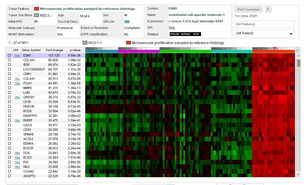
Clicking on a data point in the heatmap will populate the metadata box above the heatmap with information specific to that gene and tumor. This meta-information includes information regarding the tumor, the gene and a search box to search for genes that show similar expression patterns as your gene of interest. There are two links available from the tumor box, clicking on the “Tumor Sub-Block” link will open up a new tab with the Specimen Detail Page and clicking the “SNI” link will take you to the Swedish Neuroscience Institute page (registration is required to access the patient metadata). Gene information includes metadata on the gene selected including links to ISH data for that gene (when available) and links to other Allen Brain Atlas resources that include that gene.

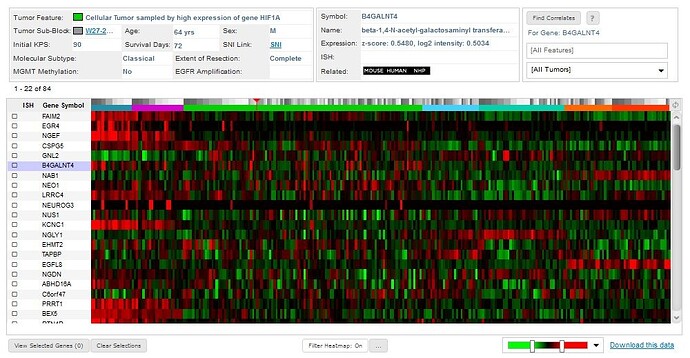
If there is ISH data available for a gene, there will be a link labeled “Yes” that will take you to the ISH Data for that gene.

You can adjust the window and the level of the color scale on the heatmap by adjusting the threshold bars or re-centering the color map scale bar. You can also zoom in or out to see the heatmap at different magnification levels.

You can select a set of genes for later viewing by selecting the check-boxes beside the list of gene symbols. Your choices are stored in a browser cookie in your computer and will remain in effect until you click the “Clear Selections” button or clear your web browser’s cookie cache. Click the “View Selections” button to see your selections.

To restrict the columns that are displayed, select the “Filter Heatmap” button below the heatmap. Filtering your heatmap is a two-step process: first, select the “…” box to restrict your features, making sure to save your selections and then toggle the filter heatmap feature by clicking the “Filter Heatmap” button.

‍

Correlative Search

In using gene expression databases, a “search by example” feature is highly desirable as genes with similar expression patterns may be related in function. Using the “Find Correlates” search utility will accomplish this function.

Once you have selected a gene of interest (by clicking on the heatmap that results from a Gene Search or Differential Search), you can find genes with similar expression patterns. All Features and All Tumors are included in your search by default, but you can select one or more features or tumors from the drop down menus. Once you have selected the tumor feature(s) and tumor(s) of interest, click “Find Correlates”.

The search results highlight the genes whose expression profiles across the samples of interest resemble the expression profile of the example gene by ranking the genes according to the Pearson’s correlation coefficient (r) between their profile and that of the example gene.

If there is ISH data available for a gene, there will be a link labeled “Yes” that will take you to the ISH Data for that gene.

You can see “anti-correlated” genes by toggling the sort order on column “r” or scrolling to the bottom of the heatmap.

‍

Differential Search

Another common usage of gene expression databases is to find genes that show enrichment of expression in one set of samples compared to another set of samples. This type of query is supported by the “Differential Search” feature. Under the RNA-Seq tab, click on the examples in the “Browse by Differential Expression” box, or select the “Differential Search” radio button to start your own search. To find genes enriched in one “target set” of tumor features and/or tumors compared to a “contrast set” of tumor features and/or tumors, choose the target set using the “Target Tumor Features/Tumors” drop down menu, and the contrast set using the “Contrast Tumor Features/Tumors” drop down menu. The default setting selects all tumor features and tumors, but clicking in the “All Features” or “All Tumors” text boxes will allow you to select individual tumor feature(s)/tumor(s). Then, click “Search”.

The search will return a list of genes enriched in the target domain(s) over the contrast domain(s) ranked by the Fold change in expression values. The results can be sorted also by the statistical significance of the evidence (p-Value) by clicking on the desired sort parameter.

‍

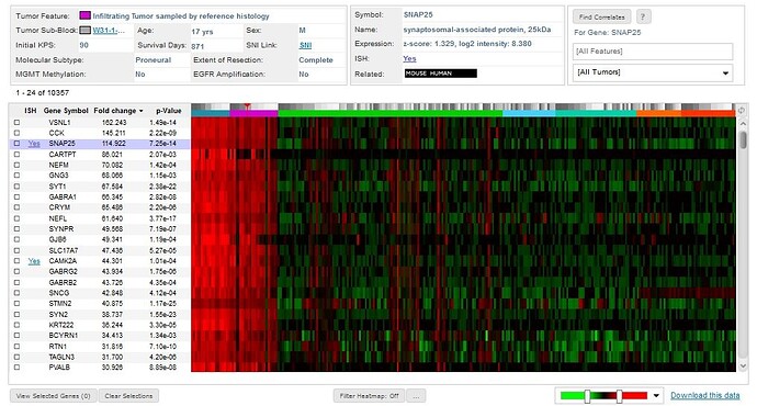
If there is ISH data available for a gene, a link labeled “Yes” takes you to the ISH Data for that gene.

‍

Download Search Results

To download your search results, click the “Download this data” link at the bottom left of the heatmap. You will have the option of downloading up to 2000 genes at a time starting from any position in the heatmap. Your start position can be determined from the counter in the top left corner of the heatmap (see screenshot).

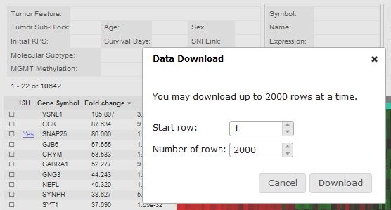
Your data will be downloaded as three separate files: 1) a Columns.csv file that lists the column headers with associated metadata for each sample, 2) a Rows.csv file that lists the row headers with associated metadata for each gene, and 3) an Expression.csv file that provides a matrix of the expression values for each data point.

The column headers, row headers and expression data will be consistent with the settings from which you downloaded the heatmap (i.e. color map).

To download the complete data set used in the heatmap, go to the Download tab and click the appropriate link.

‍

Explore More Resources

Documentation

In Situ Hybridization ISH Data For Ivy Glioblastoma Atlas Project

Learn about In Situ Hybridization ISH Data For Ivy Glioblastoma Atlas Project with comprehensive guides and examples from Allen Institute for Brain Science.

Searching the Database

Under the ISH tab, there are several ways to search the database.

‍

Specimen Search

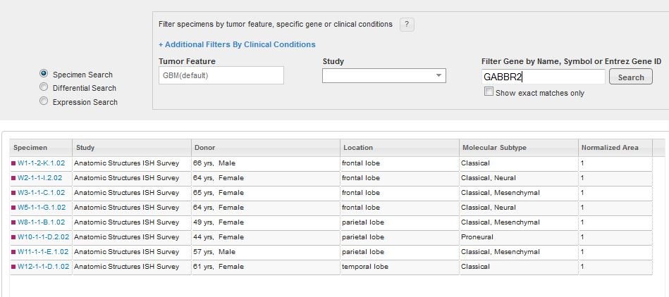
To search for a specific glioblastoma specimen type, filter your search criteria by a specific gene, tumor feature, study or specific clinical conditions.

‍

To refine your search by specific clinical conditions, click the “+” next to “Additional Filters By Clinical Conditions”.

‍

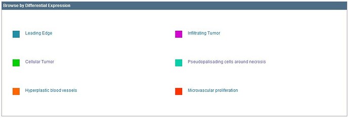
If you are unsure of where to begin your search, you can browse by the tumor information where the columns are described below.

Column	Definition
Tumor	Specimen ID of the tumor, linking to the Specimen Detail Page
Molecular Subtype	Classical: chromosome 7 amplification (EGFR), paired with chromosome 10 loss. Mesenchymal: noted for focal hemizygous deletions of a region at 17q11.2 (NF1). Proneural: defined by alterations of PDGFRA and point mutations in IDH1. Neural: typified by the expression of neuronal markers such as NEFL, GABRA1, SYT1, and SLC12A5.
Extent of Resection	Degree to which tumor tissue was surgically removed
Surgery	Whether the tumor was a primary surgery, or removal of a subsequent recurrent tumor
MGMT Methylation	A diagnostic test result referring to whether a tumor’s O-6-methylguanine-DNA methyltransferase DNA repair gene was methylated
Survival Days	Number of days from the initial diagnosis
EGFR Amplification	A diagnostic test result referring to whether a particular tumor’s epidermal growth factor receptor (EGFR) gene had multiple copies
Initial KPS	Karnofsky Performance Status is a measure of functional impairment (on a scale of 0-100, 0 referring to dead, 50 to requiring considerable assistance and frequent medical care, and 100 referring to no evidence of disease)
Age	Age in years at the time of diagnosis
SNI Link	Link to the Swedish Neurological Institute page for this donor (Registration required)

‍

Gene Search

The genes chosen for this project were selected based upon current knowledge of GBM biology and what was learned from each of the individual Ivy GAP Studies. To see a list of genes for each study, please see the Gene Lists whitepaper in Documentation. Typing in the gene search text box will bring up a list of suggested genes. If your gene of interest was not assayed in this project, no results will be returned. Once you have chosen a gene, either by selecting a gene from the suggested list, or hitting “Enter” after typing in the name, symbol or ID, a list of specimen blocks that contain search results fulfilling your criteria will open.

‍

Tumor Feature

Each of the tumor structural features was identified and labeled in ~12,000 H&E histological images using a semi-automated annotation application based on advanced statistical machine learning algorithms, and can be searched and visualized in the Ivy GAP web application.

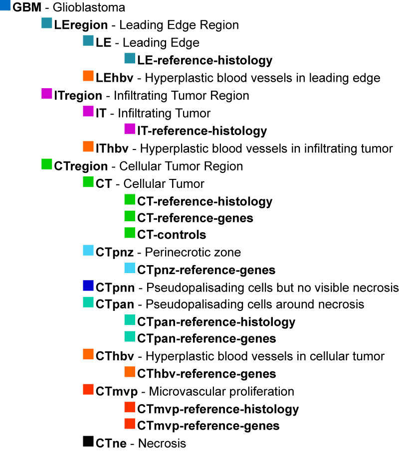
Tumor features are described using a specific ontology. The Ivy GAP ontology is a hierarchical organization of glioblastoma anatomic structural features and associated transcriptomes from RNA-Seq samples that were identified by reference histology or reference gene expression patterns. It does not reflect ontological origins of the structural features; it is simply a representation of relationships among the glioblastoma features and gene expression patterns associated with putative cancer stem cell clusters that were identified in the project.

The structural features are commonly identified by neuropathologists in glioblastoma tissue sections stained with Hematoxylin and Eosin (H&E). The major structural regions are Leading Edge (LE), Infiltrating Tumor (IT), and Cellular Tumor (CT).

Within each of these regions, particular structural features can be found such as Microvascular Proliferation (MVP), Pseudopalisading Cells around Necrosis (PAN), Hyperplastic Blood Vessels (HBV), and Necrosis (NE). These features are routinely used to distinguish glioblastoma, or Grade IV glioma, from lower grades of glioma. The feature HBV can be observed occasionally in the LE and IT regions, but it as well as MVP, NE, and PAN are frequently identified in the CT region.

‍

Specimen Search Results

Column	Description
Specimen	Clicking on this link will take you to a Specimen Detail Page
Study	Indicates which study the samples were assayed
Donor	Donor age and gender
Location	Location in the brain from which the tumor was removed
Molecular Subtype	Classical: chromosome 7 amplification (EGFR), paired with chromosome 10 loss. Mesenchymal: noted for focal hemizygous deletions of a region at 17q11.2 (NF1). Proneural: defined by alterations of PDGFRA and point mutations in IDH1. Neural: typified by the expression of neuronal markers such as NEFL, GABRA1, SYT1, and SLC12A5.
Normalized Area	The fraction of the selected “structure” in the specimen sub-block

‍

Differential Search

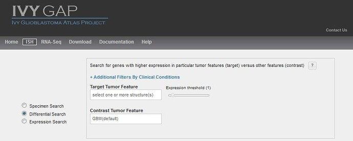
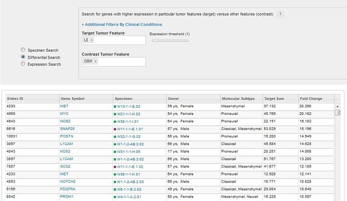
Similar to other Atlases in the Allen Brain Atlas resources, you can search for enriched gene expression in a tumor feature or structure by comparing expression between your target structure and a contrast structure. By default, this search uses all the data as contrast, but changing the contrast structure to more define your search will produce different results. Changing the threshold on a differential search will restrict the list of returned results by excluding any experiment where the expression energy of the target structures is less than threshold.

Several differential searches have already been calculated for you and are accessible by selecting from the “Browse by Differential Expression”.

Differential Search Results

Performing a differential search will return a list of specimen blocks that include the genes with the highest differential expression levels ranked by fold change in the target structure over the contrast structure.

‍

Column Header	Description
Entrez ID	Unique identifier from the National Center for Biotechnology Information (NCBI) database for gene-specific information
Gene Symbol	The gene symbol, which is a short abbreviated form of the gene name. Clicking on this link will take you to all GBM experiments performed on this gene
Specimen	Clicking on this link will take you to a Specimen Detail Page
Donor	Donor age and gender
Molecular Subtype	Classical: chromosome 7 amplification (EGFR), paired with chromosome 10 loss. Mesenchymal: noted for focal hemizygous deletions of a region at 17q11.2 (NF1). Proneural: defined by alterations of PDGFRA and point mutations in IDH1. Neural: typified by the expression of neuronal markers such as NEFL, GABRA1, SYT1, and SLC12A5.
Target Sum	Sum of gene expression energy over all the target structures
Fold Change	The measure describing how gene expression changes when comparing the target structure(s) expression energy to the contrast structure(s) expression energy

‍

Expression Search

‍

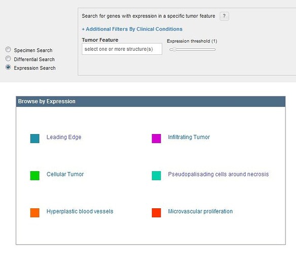
To see gene expression ranked by expression energy within a single glioblastoma structure, use the Expression Search feature. Clicking on a tumor feature from the Glioblastoma Ontology or the “Browse by Expression” box will return a list of genes ranked by the average expression where each column is described below.

Column	Description
Entrez ID	Unique identifier from the National Center for Biotechnology Information (NCBI) database for gene-specific information
Gene Symbol	The official gene symbol, which is a short abbreviated form of the gene name. Clicking on this link will take you to all GBM experiments performed on this gene
Specimen	Clicking on this link will take you to a Specimen Detail Page
Donor	Donor age and gender
Molecular Subtype	Classical: chromosome 7 amplification (EGFR), paired with chromosome 10 loss. Mesenchymal: noted for focal hemizygous deletions of a region at 17q11.2 (NF1). Proneural: defined by alterations of PDGFRA and point mutations in IDH1. Neural: typified by the expression of neuronal markers such as NEFL, GABRA1, SYT1, and SLC12A5.
Average Expression	The sum of expressing pixels divided by sum product of pixels of that tumor feature

‍

Clinical Conditions

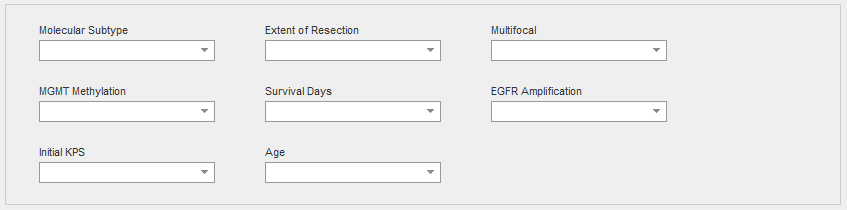
When searching for specific images, one of the search tools available to you is to “Filter by Clinical Condition”. Each condition and its significance is outlined below. Listed references can be found in the Overview whitepaper in Documentation.

‍

Molecular Subtype

Genomic characteristics of tissue block related to classification of patients. The molecular subtype was determined using all cellular tumor samples from a given tumor. An analysis of each cellular tumor sample was conducted with 840 transcripts from the RNA-Seq data as per Verhaak et al., 2010. For a given tumor, if multiple cellular tumor samples exhibited distinct subtypes, then the tumor was classified as a mixture of its subtypes. The Classical subtype refers to chromosome 7 amplification, specifically EGFR, paired with chromosome 10 loss. The Mesenchymal subtype is noted for focal hemizygous deletions of a region at 17q11.2, containing the gene NF1. The Proneural subtype is defined by alterations of PDGFRA and point mutations in IDh2. The Neural subtype is typified by the expression of neuronal markers such as NEFL, GABRA1, SYT1, and SLC12A5.

‍

Extent of Resection

Degree to which tumor tissue was surgically removed. Complete resection is associated with increased survival rates (Keles et al., 1999).

‍

Multifocality

Whether a tumor was comprised of single or multiple masses. Increased multifocality is associated with decreased rates of survival (Thomas et al., 2013).

‍

MGMT Methylation

A diagnostic test result referring to whether a tumor’s O-6-methylguanine-DNA methyltransferase DNA repair gene was methylated. Methylated MGMT is associated with increased rates of survival (Hegi et al., 2013).

‍

Survival Days

Patient’s lifespan since initial diagnosis

‍

EGFR Amplification

A diagnostic test result referring to whether a particular tumor’s epidermal growth factor receptor gene had multiple copies. The gene is frequently amplified in glioblastoma (Hobbs et al., 2012).

‍

Initial KPS

Karnofsky Performance Status when first diagnosed with first tumor. Karnofsky Performance Status is a measure of functional impairment on a scale of 0-100, 0 referring to dead, 50 to requiring considerable assistance and frequent medical care, and 100 referring to no evidence of disease. High scores are associated with increased survival rates (Ening et al., 2015).

‍

Age

Patient age in years at time of diagnosis. Younger patients tend to have increased survival rates (Ening et al., 2015).

‍

Specimen Detail Page

‍

Donor Page

Clicking on a Specimen ID will bring you to the specimen detail page.

Tumor Subdivision - Navigation of tumor subdivisions and button for viewing patient and tumor summary information. the color in a tissue sub-block indicates the study in which the sub-block was used.
Tumor Features in this Sub-Block - The glioblastoma tumor features that were identified and assayed for in the yellow highlighted sub-block. The color coding corresponds to the glioblastoma ontology.
ISH Image - An image viewer showing the in situ hybridization experiment, and related features.
Nearest H&E Image - Image and annotated anatomic tumor features of a nearby H&E stained tissue section.
Section Information - Lists the Gene, Experiment ID, Section #, Treatments, and the study.
Genes Surveyed in this Sub-Block - All genes assayed in this specimen sub-block are listed. To view a specific gene, select only that gene from the list.
Selection Cart - When viewing an ISH image, select the checkbox to add the image to your viewing cart. Images selected in your cart are available to view until the cache is cleared or you click “Clear Selections”.

‍

Patient, Tumor and MRI Summary

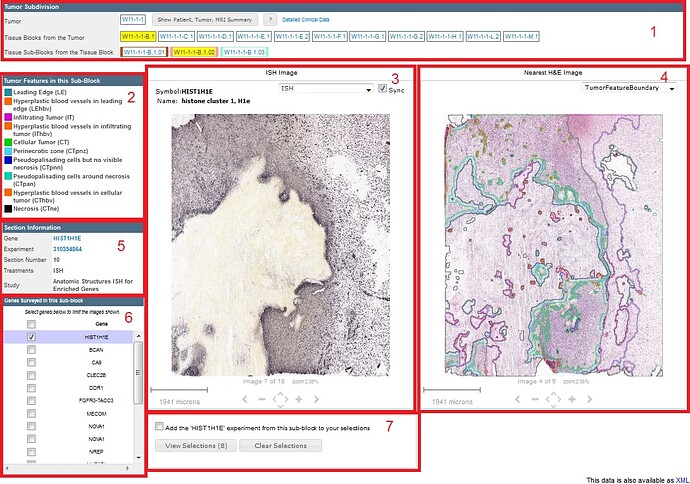
This panel displays information on patient and tumor, and on how the tumor was subdivided into blocks. This panel is arrived at by toggling the “View Patient, Tumor and MRI Summary” button in the Tumor Subdivision section of the Specimen Detail Page.

‍

Description of Donor ID

The tumor names (or IDs) identify tumors across the different resources associated with the Ivy Glioblastoma Atlas Project. In the name W1-1-2, W1 identifies the patient, and -1-2 indicate that this tumor was the second mass removed during the first surgery.

The names of the tumor blocks were assigned as indicated in the Resected Tumor Image, and the names of the sub-blocks reflect their position within the tumor block.

‍

Image Viewer

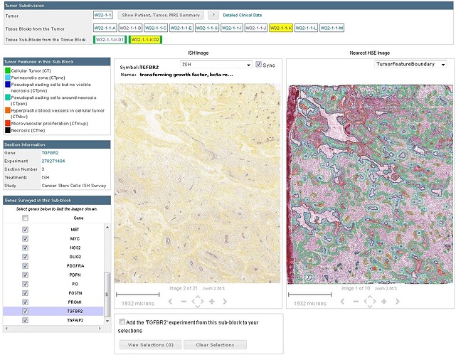
The GBM image viewer allows you to navigate through a series of specimen sub-block ISH images to view at higher resolution. Once a gene image is selected, you can manipulate it with your mouse and use the keyboard or on screen navigation tools to take additional actions.

The gene symbol and gene name are displayed in the title bar along with a dropdown menu and a “Sync” feature to allow you to navigate and keep the adjacent H&E viewer synched with your movements. The dropdown menu allows you to view the ISH image, the Expression Mask, the annotated features, or the annotated feature boundaries. If all the genes are selected in Box #6, the entire specimen sub-block can be viewed using the onscreen navigation tools or the keyboard commands. The current selection is outlined in black.

To view images at high resolution, in the Section Information box, click on the Experiment link; then, click the icon in the upper right corner of the viewer. Use the dropdown menu to select the type of image you want to see.

Alternatively, to view all the images available for a given gene, in the Section Information box, click on the gene symbol link.

‍

Scale Bar

Shows the current viewing resolution of the image, in microns. This value dynamically changes as you zoom in/out of the image. You can position the scale bar anywhere on the main image by dragging the scale bar by its ruler.

You can toggle the orientation of the scale bar from horizontal to vertical by clicking on the scale bar text.

‍

Keyboard Commands

Key	Description
F	Advance to the next image from the specimen
D	Go back to the previous image from the specimen
R	Advance to the last image in the series
E	Go back to the first image in the series
A	Zoom in
Z	Zoom out

‍

Expression Mask Colors

The Expression mask image display highlights those cells that have the highest probability of gene expression using a heatmap color scale (from low/blue to high/red).

Learn more

API

API For Ivy Glioblastoma Atlas Project

Learn about API For Ivy Glioblastoma Atlas Project with comprehensive guides and examples from Allen Institute for Brain Science.

The Ivy Glioblastoma Atlas Project (Ivy GAP) is a foundational resource for exploring the anatomic and genetic basis of glioblastoma at the cellular and molecular levels.

Six studies were designed to identify the molecular signatures and measure heterogeneity. In Situ Hybridization (ISH) was used to screen for gene expression enriched in particular structures and cell clusters, and laser microdissection followed by RNA sequencing were used to generate the transcriptomes and identify the genetic markers.

Overall, the dataset spans 42 individual tumors. Each tumor was sub-divided into sub-blocks for processing in one of the six studies. See whitepapers for more details about the tumor specimens, tissue and informatics processing.

From the API, you can:

Download images

Download quantified ISH expression values by tumor feature

Query the ISH expression differential search services

Download RNA-Seq expression values

Query the RNA-Seq correlative and differential search services

This document provides a brief overview of the data, database organization and example queries. API database object names are in camel case. See the main API Documentation for more information on data models and query syntax.

‍

ISH Surveys

‍

Experimental Overview and Metadata

Experimental data from the four ISH surveys is associated with the “Glioblastoma” Product.

Multiple genes were assayed using each sub-block Specimen. The Specimen is cryosectioned into 20µm thick sections. ISH sections are interleaved with H&E sections such that every ISH is adjacent to an H&E section, yielding a single image SectionDataSet for each gene and one H&E SectionDataSet with 11-15 images.

Each sub-block Specimen is associated with a SpecimenType identifying the study to which this sub-block belongs.

Each H&E section is processed through a semi-automated annotation application that labels anatomic features using a statistical machine learning algorithm. The algorithm associates each 45x45 pixel neighborhood to a tumor feature label. Additionally, a separate algorithm counts the number of nuclei and the nuclei fraction coverage within each neighborhood.

Tumor feature statistics for each sub-block Specimen are generated by summing up the 45x45 pixel neighborhoods over all H&E images. This process produces area, normalized area, nuclei count, and nuclei fraction coverage for each sub-block Specimen and feature of interest.

Anatomic tumor features (also referred to as structures) are hierarchically organized into a tree in which a child structure is a “part of” its parent structure. Structures are assigned colors to visually emphasize their relationships in the hierarchy. See the structure ontology page for more information.

Examples:

All donors in the “Glioblastoma” Product

‍

http://api.brain-map.org/api/v2/data/query.xml?criteria= model::Donor, rma::criteria,products[name$eq'Glioblastoma']

‍

All sub-block Specimens which are part of the “Anatomic Structures ISH Survey”

‍

http://api.brain-map.org/api/v2/data/query.xml?criteria= model::Specimen ,rma::criteria,specimen_types[name$eq'Anatomic Structures ISH Survey'] ,rma::options[num_rows$eqall]

‍

All TumorFeatures in sub-block Specimen “W32-1-1-K.01”

‍

http://api.brain-map.org/api/v2/data/query.xml?criteria= model::TumorFeature ,rma::criteria,data_set(specimen[external_specimen_name$eq'W32-1-1-K.01']) ,rma::include,structure

‍

All ISH SectionDataSets in sub-block Specimen “W32-1-1-K.01”

‍

http://api.brain-map.org/api/v2/data/query.xml?criteria= model::SectionDataSet ,rma::criteria,specimen[external_specimen_name$eq'W32-1-1-K.01'],treatments[name$eq'ISH'] ,rma::include,genes,sub_images

‍

From the above query, specimen “W32-1-1-K.01” has 21 ISH SectionDataSet (id=278269453 is one of them). In the web application, images from a specimen are displayed in a specimen page. All displayed information, images and structural expression values are also available through the API.

See the image download page to learn how to download images at different resolutions and regions of interest.

SpecimenPage — **Figure**: Specimen page of specimen “W32-1-1-K.01” showing all 21 ISH SectionDataSet on the left image panel and 10 H&E images on the right image panel. The color codes for the anatomic tumor features outlined in the H&E images are displayed on the left.

‍

ISH Expression Quantification

For every ISH image, pixels with gene expression are detected and a grayscale mask generated. The detection algorithm is based on adaptive thresholding and mathematical morphology. Then the ISH image is registered to its closet H&E image using a multi-resolution elastic registration algorithm. Finally, feature label and nuclei count information is transferred from 45x45 pixel neighborhood in the H&E image onto the expression data.

Expression statistics for each tumor feature are computed by combining values from all the neighborhoods with the same label. This process produces expression density, intensity and energy measurements for each experiment and anatomical feature. For an anatomical feature, expression energy is defined as sum of expressing pixel divided by sum product of pixels in each neighborhood label for that feature and its nuclei fraction coverage.

Examples:

Download tumor feature expression values for POSTN SectionDataSet (id=265857641) in sub-block “W8-1-1-E.1.03”

‍

http://api.brain-map.org/api/v2/data/query.xml?criteria= model::StructureUnionize ,rma::criteria,section_data_set[id$eq265857641] ,rma::include,structure

‍

ISH Expression Search Service

The expression search service allows users to instantly search over the ~18000 SectionDataSets to find genes with specific expression patterns:

The Expression Search function allows users to find genes which expression in one structure (or set of structures)
The Differential Search function allows users to find genes which have higher expression in one structure (or set of structures) compared to another structure (or set of structures)

The expression search functionality is available through the Web application and the API.

To perform an Expression Search, a user specifies a set of target structures. For each StructureDataSet, the average expression energy is computed for the target structures. The returned results are sorted in descending order of average expression energy.

See the connected service page for definitions of service::gbm_ish_expression parameters

Examples:

Find genes (SectionDataSets) with expression in pseudopalisading cells around necrosis (CTpan)

‍

http://api.brain-map.org/api/v2/data/query.xml?criteria= service::gbm_ish_expression[structures$eqCTpan][threshold$eq0,100000]

‍

Find genes (SectionDataSets) with expression in hyperplastic blood vessels (LEhbv, IThbv, CThbv)

‍

http://api.brain-map.org/api/v2/data/query.xml?criteria= service::gbm_ish_expression[structures$eqLEhbv,IThbv,CThbv][threshold$eq0,100000]

‍

Visualize expression search in the web application

To perform a Differential Search, a user specifies a set of target structures and a set of contrast structures. For each StructureDataSet, the sum expression energy is computed for the target structures and for the contrast structures. The returned results are sorted in descending order of the ratio of the sum expression energy of the target structures over the sum expression energy of the contrast structures.

See the connected service page for definitions of service::gbm_ish_differential parameters

Examples:

Find genes (SectionDataSets) with higher expression in pseudopalisading cells around necrosis (CTpan) than cellular tumor cells (CT)

‍

http://api.brain-map.org/api/v2/data/query.xml?criteria=service::gbm_ish_differential [structures1$eqCT][structures2$eqCTpan][threshold1$eq0,100000][threshold2$eq1,100000]

‍

Find genes (SectionDataSets) with higher expression in infiltrating tumor (IT) than cellular tumor (CT) and leading edge (LE)

‍

http://api.brain-map.org/api/v2/data/query.xml?criteria=service::gbm_ish_differential [structures1$eqIT,CT][structures2$eqIT][threshold1$eq0,100000][threshold2$eq1,100000]

‍

Visualize expression search in the web application

It should be noted that the expression quantification values used by the search services are generated by a fully automated processing pipeline. False positive and false negative results can occur due to artifacts on the tissue section or slide and/or algorithmic inaccuracies. Users should confirm results by visually inspecting the ISH images.

‍

RNA-Seq Surveys

‍

Experimental Overview and Metadata

Experimental data from the two RNA-Seq surveys is associated with the “Human Glioblastoma RNASeq” Product.

For the “Anatomic Structures RNA-Seq” study, sampling locations were manually identified after H&E staining. For the “Cancer Stem Cells RNA-Seq”, 17 reference gene probes were used to identify 35 types of putative cancer stem cell clusters.

Each sampling site is associated with a Structure with the following naming scheme:

XX-reference-histology: tumor feature XX sampled by reference histology
XX-reference-genes: tumor feature XX sampled by reference gene(s)
XX-reference-controls: tumor feature XX sampled by low expression of reference genes

Structures are organized hierarchically into a tree in which children structures are “parts of” their parent structure. Structures are assigned colors that visually emphasize the hierarchical relationships. See the structure ontology page for more information.

See whitepapers for more details about the RNA-Seq data generation and normalization. All gene and sampling site information can be accessed through the API.

Examples:

All donors in the “Human Glioblastoma RNASeq” Product

‍

http://api.brain-map.org/api/v2/data/query.xml?criteria= model::Donor, rma::criteria,products[name$eq'Human Glioblastoma RNASeq']

‍

All samples in the “Human Glioblastoma RNASeq” Product

‍

http://api.brain-map.org/api/v2/data/query.xml?criteria= model::Sample ,rma::criteria,tissue_sample_data_set(products[name$eq'Human Glioblastoma RNASeq']) ,rma::include,structure,tissue_sample_data_set(specimen(donor)) ,rma::options[num_rows$eqall]

‍

RNA-Seq Expression Download Service

Normalized gene-level expression values can be downloaded in several ways:

From the web application Download page
From the connected data service in the API

Using the connected service, expression values can be obtained by specifying:

a list of “probes” (genes),
a list of “donors” (tumor specimens, optional), and
a list of structures (optional)

See the connected service page for definitions of service::gbm_expression parameters.

Example:

Download expression values for gene ESM1 restricted to samples from tumor ‘W1-1-2’

Find Specimen ID for tumor ‘W1-1-2’ (id=703393)

‍

http://api.brain-map.org/api/v2/data/query.xml?criteria= model::Specimen ,rma::criteria,[external_specimen_name$eq'W1-1-2']

‍

Find Gene ID for human gene ESM1 (id=10924)

‍

http://api.brain-map.org/api/v2/data/query.xml?criteria= model::NcbiGene ,rma::criteria,[acronym$eqESM1],organism[name$eq'Homo Sapiens']

‍

Use tumor and gene ID as parameters to service::gbm_expression

‍

http://api.brain-map.org/api/v2/data/query.xml?criteria= service::gbm_expression[probes$eq10924][donors$eq703393]

‍

The output of the service has two top level ordered arrays “probes” and “samples”. For example:

‍

“probes”:[{“id”:10924, “name”:“endothelial cell-specific molecule 1”, “gene-id”:10924, “gene-symbol”:“ESM1”,“gene-name”:“endothelial cell-specific molecule 1”, “entrez-id”:11082,“chromosome”:“5”,“start-position”:“n/a”,“end-position”:“n/a”, “expression_level”:[“1.0498”,“0.3790”,“0.1323”,“0.1894”,“0.2724”,“0.0268”,“0.0000”,“1.3249”,“1.0818”,“0.9904”,“1.4085”,“0.0301”,“0.0000”,“0.6687”,“6.9482”,“7.9008”,“6.8374”,“8.5132”], “z-score”:[“-0.6017”,“-0.8612”,“-0.9566”,“-0.9345”,“-0.9024”,“-0.9974”,“0.0000”,“-0.4953”,“-0.5893”,“-0.6247”,“-0.4630”,“-0.9961”,“0.0000”,“-0.7491”,“1.6797”,“2.0481”,“1.6368”,“2.2850”]} ],“samples”:[ {“donor”:{“id”:703393,“name”:“W1-1-2”,“age”:“”,“color”:“646464”},“sample”:{“well”:300629386,“polygon”:298763268,“mri”:[-1,-1,-1]}, “structure”:{“id”:298764274,“name”:“Leading Edge sampled by reference histology”,“abbreviation”:“LE-reference-histology”,“color”:“218FA5”}, “top_level_structure”:{“id”:9429,“name”:“Glioblastoma”,“abbreviation”:“GBM”,“color”:“006EC6”}}, {“donor”:{“id”:703393,“name”:“W1-1-2”,“age”:“”,“color”:“646464”},“sample”:{“well”:300629325,“polygon”:298726093,“mri”:[-1,-1,-1]}, “structure”:{“id”:298764274,“name”:“Leading Edge sampled by reference histology”,“abbreviation”:“LE-reference-histology”,“color”:“218FA5”}, “top_level_structure”:{“id”:9429,“name”:“Glioblastoma”,“abbreviation”:“GBM”,“color”:“006EC6”}}, {“donor”:{“id”:703393,“name”:“W1-1-2”,“age”:“”,“color”:“646464”},“sample”:{“well”:300173638,“polygon”:298727595,“mri”:[-1,-1,-1]}, “structure”:{“id”:298764274,“name”:“Leading Edge sampled by reference histology”,“abbreviation”:“LE-reference-histology”,“color”:“218FA5”}, “top_level_structure”:{“id”:9429,“name”:“Glioblastoma”,“abbreviation”:“GBM”,“color”:“006EC6”}}, … ],

‍

Each probe (Gene) contains information about:

the Gene (id, name)
the associated NCBI Gene (id, acronym, name, entrez-id), along with
a vector of normalized expression values and z-scores in the same order as the “samples” array.

Each sample contains information about:

the Tumor (id and name returned in the “donor” field)
the associated Structure (id, name, acronym and color)

‍

RNA-Seq Expression Search Service

‍

Differential Search

The Differential Search finds genes that show the greatest difference in expression values between two sets (target and contrast) of user-defined structures. For each probe, a 2-sample t-test is performed followed by a Benjamini and Hochberg false discovery rate correction. The null hypothesis is that the average expression level of samples in the contrast set of structures is greater than or equal to the average expression level of samples in the target set of structures. A statistically significant result (p-value less than user-defined threshold) allows us to reject the null hypothesis and conclude that the average expression level of samples in the target set of structures is greater than the average expression level of samples in the contrast set of structures. Resulting p-values are sorted in ascending order. Search results can also be sorted by fold-change (log ratio of expression) in descending order.

The differential search functionality is available through the Web application and the API.

See the connected service page for definitions of service::gbm_differential parameters.

Example:

Differential search for genes with higher expression in microvascular proliferation (sampled by reference histology) than in cellular tumor, infiltrating tumor, leading edge and pseudopalisading cells around necrosis.

‍

http://api.brain-map.org/api/v2/data/query.xml?criteria= service::gbm_differential [structures1$eq'CT-reference-histology','IT-reference-histology','LE-reference-histology','CTpan-reference-histology'] [structures2$eq'CTmvp-reference-histology'][sortby$eq'fold-change']

‍

Visualize differential search results in the web application

DifferentialSearch — **Figure**: Screenshot of top returns of a differential search for genes with higher expression in microvascular proliferation.

Correlative Search

The Correlative Search finds genes with expression profiles similar to that of a selected seed “probe” over all samples within a user-specified structure and for user-specified tumors/donors. Pearson’s correlation coefficients are computed for all probes and the results ranked in descending order.

The correlative search functionality is available through the Web application and the API.

See the connected service page for definitions of service::gbm_correlation parameters.

Example:

Correlative search for genes with a similar expression to gene VEGFA (id=7379) over all samples

‍

http://api.brain-map.org/api/v2/data/query.xml?criteria= service::gbm_correlation[probes$eq7379][structures$eqGBM]

Learn more

Document Collection

Documentation Ivy Glioblastoma Atlas Project

Learn about Documentation Ivy Glioblastoma Atlas Project with comprehensive guides and examples from Allen Institute for Brain Science.

Available Files

‍

Learn more