MapMyCells Use case: single cell genomics in mouse
Overview
Click here to download the full R notebook for your own use
MapMyCells enables mapping of single cell and spatial trancriptomics data sets to a whole mouse brain taxonomy. The taxonomy is derived and presented in “A high-resolution transcriptomic and spatial atlas of cell types in the whole mouse brain” (https://www.biorxiv.org/content/10.1101/2023.03.06.531121v1), and we encourage you to cite this work if you use MapMyCells to transfer these labels to your date. This R workbook illustrates a common use case for the MapMyCells facility (https://knowledge.brain-map.org/mapmycells/process/) and follow up analyses. The query data included in this document are from the paper “The cell type composition of the adult mouse brain revealed by single cell and spatial genomics” (https://doi.org/10.1101/2023.03.06.531307) from the Chen and Macosko labs, which also has a nice data exploration tool (Brain Cell Data Viewer; https://docs.braincelldata.org/).
Prepare your workspace
Install R and (optionally RStudio)
This example is run and R, which can be downloaded at CRAN (https://cran.r-project.org/). To run in R, just sequentially copy and paste the relevant code blocks into R. An easier alternative is to download RStudio here (https://posit.co/download/rstudio-desktop/) after downloading R. “.Rmd” files can be directly loaded into R studio and run.
Prior to running any code, download the data:
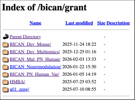
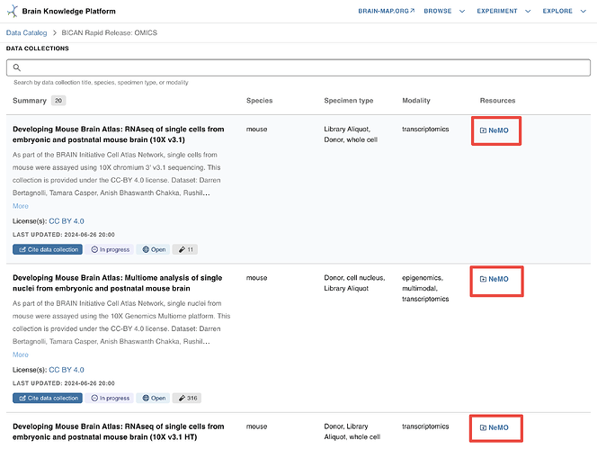
To get started first download an example 10x library from the paper above. We choose data from primary motor cortex (MOp) to apply knowledge from the series of 2021 BICCN studies at https://www.biccn.org/cell-census-primary-motor-cortex. Extract the file below from the NeMO archive to your working directory: https://data.nemoarchive.org/biccn/grant/u19_huang/macosko_regev/transcriptome/sncell/10X_v2/mouse/processed/counts/pBICCNsMMrMOPi70470511Bd180328.mex.tar.gz Unzipping will produce a folder called “pBICCNsMMrMOPi70470511Bd180328” with three files: “Matrix.mtx”, “barcodes.tsv”, and “genes.tsv”. This is the standard output for a single 10X run (and other droplet-based methods), and data can be read in using standard R scripts. The MOP in the file name indicates that this particular library is from a primary motor cortex dissection.
Now you are ready to start R (or RStudio).
Set the working directory
The next component of set up is to make sure your R working directory points to the data you are reading in.
# Uncomment line below and replace bracketed text with path to downloaded files.
#setwd("FILE_PATH")
Load the relevant libraries
This workbook uses the libraries anndata and Seurat.
# Install Seurat and anndata if needed
list.of.packages <- c("Seurat", "anndata")
new.packages <- list.of.packages[!(list.of.packages %in% installed.packages()[,"Package"])]
if(length(new.packages)>0) install.packages(new.packages)

# Load Seurat and anndata
suppressPackageStartupMessages({
  library(Seurat)      # For reading droplet data sets and visualizing/comparing results
  library(anndata)     # For writing h5ad files
})Warning: package ‘Seurat’ was built under R version 4.2.3Warning: package ‘anndata’ was built under R version 4.2.3options(stringsAsFactors=FALSE)

# Citing R libraries# citation("Seurat")
# Note that the citation for any R library can be pulled up using the citation command. We encourage citation of R libraries as appropriate.
With the above files in your current working directory and the above libraries loaded, the use case below can now be run.
Analysis of a library
(If you already have an .h5ad file ready for upload, skip to step 4.)
A common use case for analysis of single cell/nucleus transcriptomics is to collect data from one (or more) ports of a droplet-based scRNA-seq run. After some QC steps, these are then clustered for defining cell types. This section describes how to start from a such a droplet-based sequencing run, transfer labels from mouse “10x scRNA-seq whole brain” data from the Allen Institute onto these cells using MapMyCells, and then visualize the results in a UMAP.
1. Read library data into R
10x (and other droplet-based) output includes files for the cells (“barcodes.tsv”), the genes (“genes.tsv”), and the corresponding reads (“matrix.mtx”). These can be read into a sparse matrix in R with appropriate formatting using the function “Read10X”.
dataIn <- Read10X("pBICCNsMMrMOPi70470511Bd180328/")
dim(dataIn)[1]  27998 737280
This reads in a data matrix with >700,000 columns as potential cells. However, this includes all of the empty wells.
2. QC data
For demonstrative purposes, we will define all barcodes with >250 reads as interesting “cells”, but in a real experiment more careful QC is strongly encouraged.
dataQC <- dataIn[,colSums(dataIn)>250]
dim(dataQC)[1] 27998  3673
This brings the input library down to a more reasonable ~3600 cells.
3. Output to h5ad format
Now let’s output the QC’ed data matrix into an h5ad file and output it to the current directory for upload to MapMyCells. Note that in anndata data structure the genes are saved as columns rather than genes so we need to transpose the matrix first.
# Transpose data
dataQCt = Matrix::t(dataQC)

# Convert to anndata format
ad <- AnnData(
  X = dataQCt,
  obs = data.frame(group = rownames(dataQCt), row.names = rownames(dataQCt)),
  var = data.frame(type = colnames(dataQCt), row.names = colnames(dataQCt))
)

# Write to compressed h5ad file
write_h5ad(ad,'droplet_library.h5ad',compression='gzip')

# Check file size. File MUST be <500MB to upload for MapMyCells
print(paste("Size in MB:",round(file.size("droplet_library.h5ad")/2^20)))[1] "Size in MB: 14"
If you have trouble accessing or running the previous block, check your Python accessibility in R and consider installing python as shown below. If you use Windows, you may be asked to install git before installing python, which can be accessed here: https://git-scm.com/download/win/.
library(reticulate)
version <- "3.9.12"
install_python(version)
virtualenv_create("my-environment", version = version)
use_virtualenv("my-environment")
4. Assign cell types using MapMyCells
These next steps are performed OUTSIDE of R in the MapMyCells web application.
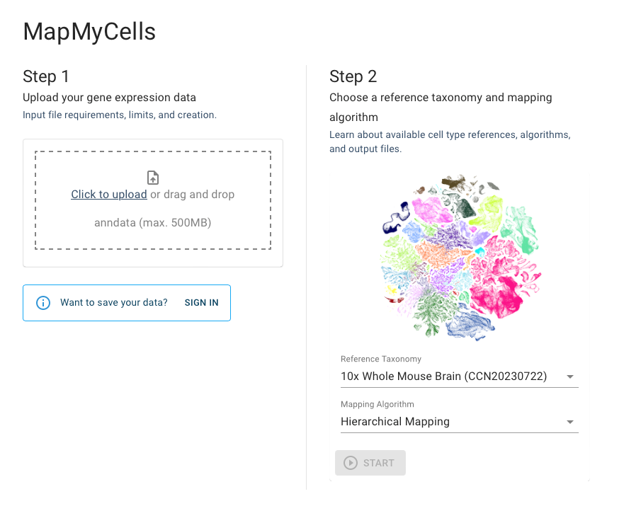
The steps to MapMyCells are as follows:
- Go to (https://knowledge.brain-map.org/mapmycells/process/).
- (Optional) Log in to MapMyCells.
- Upload ‘droplet_library.h5ad’ to the site via the file system or drag and drop (Step 1).
- Choose “10x Whole Mouse Brain (CCN20230722)” as the “Reference Taxonomy” (Step 2).
- Choose the desired “Mapping Algorithm” (in this case “Hierarchical Mapping”).
- Click “Start” and wait ~5 minutes. (Optional) You may have a panel on the left that says “Map Results” where you can also wait for your run to finish.
- When the mapping is complete, you will have an option to download the “tar” file with mapping results. If your browser is preventing popups, search for small folder icon to the right URL address bar to enable downloads.
- Unzip this file, which will contain three files: “validation_log.txt”, “[NUMBER].json”, and “[NUMBER].csv”. [NUMBER].csv contains the mapping results, which you need. The validation log will give you information about the the run itself and the json file will give you extra information about the mapping (you can ignore both of these files if the run completes successfully).
- Copy [NUMBER].csv to your current working directory and rename it “droplet_library_mapping.csv”).
- You can now go back to R and continue the script below.
5. Read mapping results into R
Let’s now look at the output results from the hierarchical clustering algorithm. We can read this into R using read.csv, but note that the first four lines contain metadata that need to be skipped.
mapping <- read.csv("droplet_library_mapping.csv",comment.char="#")
head(data.frame(mapping))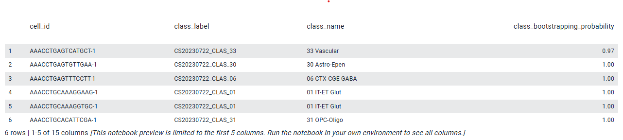
MapMyCells maps input cells to the taxonomy at four increasing levels of resolution from coarsest class, to intermediate subclass, and supertype, and finest cluster. In the mouse whole brain taxonomy there are 32 classes, 306 subclasses, 1,045 supertypes and 5,200 clusters.
The file consists of the following columns:
- cell_id = the cell identifiers for your cells included in the initial h5ad files
- class_label = the unique identifier for the best mapping class
- class_name = the name of the best mapping class
- class_bootstrapping_probability = fraction of bootstrapping runs that the cell mapped to the above class (higher numbers are better, with 1 being the best)
and similar fields for subclass, supertype, and cluster. For finest level cluster there is an additional field - cluster_alias = another unique identifier for the cluster
6. Review top classes
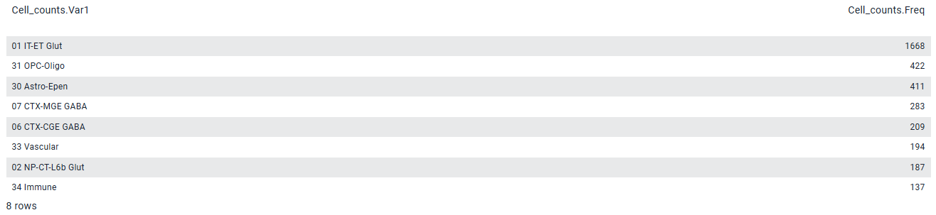
As this library was selected from a dissection of primary motor cortex (MOp), we expect the majority of cells to map to cell types found in MOp. Let’s check!\
# View the top 8 classes
data.frame(Cell_counts=head(sort(table(mapping$class_name),decreasing=T),8))
# What fraction of all cells does this represent
sum(t(t(head(sort(table(mapping$class_name),decreasing=T),8))))/length(mapping$class_name)[1] 0.9558944
The 8 most common mapped classes representing >95% of cells are glutamatergic, GABA-ergic or non-neuronal types known to be present in MOp from many published studies.
7. Visualize mapping results
To visualize the mapping results, we need both the mapping results and the original query cellxgene matrix for comparison. If this is not already read in, you can read it in from the anndata object uploaded to MapMyCells.
# Since the query data corresponds to dataQC above, we will call it dataQC again
dataQC_h5ad <- read_h5ad('droplet_library.h5ad')dataQC <- t(as.matrix(dataQC_h5ad$X))
rownames(dataQC) <- rownames(dataQC_h5ad$var)
colnames(dataQC) <- rownames(dataQC_h5ad$obs)
Now let’s visualize the mapping results. We will do this by saving the data in a Seurat object with (modified) mapping results as metadata, running the standard pipeline for creating a UMAP in Seurat, and then color-coding each cell.
# Assign rare classes and subclasses as "other"
mapping$class_new <- mapping$class_name
mapping$class_new[!is.element(mapping$class_name,names(head(-sort(-table(mapping$class_name)),8)))] = "other"
mapping$subclass_new <- mapping$subclass_name
mapping$subclass_new[!is.element(mapping$subclass_name,names(head(-sort(-table(mapping$subclass_name)),20)))] = "other"

# Put row.names as data colnames and the order to match the data
rownames(mapping) <- mapping$cell_id
mapping <- mapping[colnames(dataQC),]

# Create the Seurat object
dataSeurat <- CreateSeuratObject(counts = dataQC, meta.data = mapping)

# Standard Seurat pipeline
dataSeurat <- NormalizeData(dataSeurat, verbose = FALSE)
dataSeurat <- FindVariableFeatures(dataSeurat, verbose = FALSE)
dataSeurat <- ScaleData(dataSeurat, verbose = FALSE)
dataSeurat <- RunPCA(dataSeurat, verbose = FALSE)
dataSeurat <- RunUMAP(dataSeurat, dims = 1:10, verbose = FALSE)
Now let’s make the plot for classes!
DimPlot(dataSeurat, reduction = "umap", group.by="class_new", label=TRUE) + NoLegend()
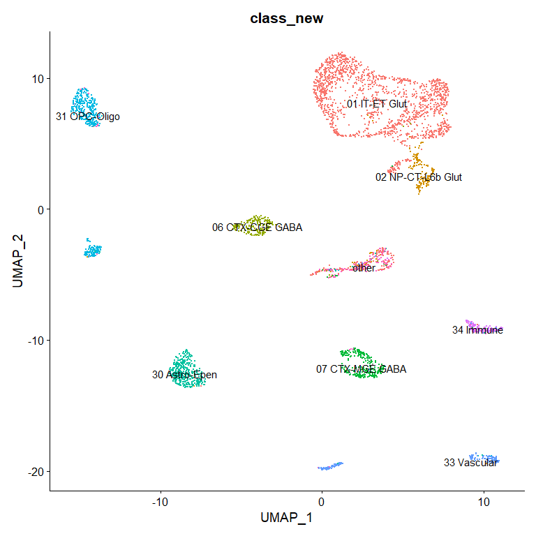
Here the data has not been clustered but rather the class assignments are assigned to the data in the UMAP. The alignment suggests that the label transfer works well. It’s worth noting that Seurat produces different UMAP configurations in different R environments, so your plot may not look exactly like this.
Now let’s make the plot where we color-code the same UMAP by subclass.
DimPlot(dataSeurat, reduction = "umap", group.by="subclass_new", label=TRUE) + NoLegend()
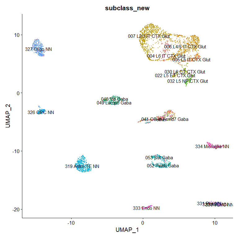
Once again, the subclasses shown largely segregate from one another without the need to apply clustering, suggesting this mapping works well even at higher resolutions. Scripts such as this can be used for visualizing and comparing mapping results.
To output the session information we write the command, which is useful for reproducibility, especially for more complex scripts.
sessionInfo()R version 4.2.2 (2022-10-31 ucrt)
Platform: x86_64-w64-mingw32/x64 (64-bit)
Running under: Windows 10 x64 (build 19045)

Matrix products: default

locale:
[1] LC_COLLATE=English_United States.utf8  LC_CTYPE=English_United States.utf8    LC_MONETARY=English_United States.utf8 LC_NUMERIC=C
[5] LC_TIME=English_United States.utf8

attached base packages:
[1] stats     graphics  grDevices utils     datasets  methods   base

other attached packages:
[1] anndata_0.7.5.6    SeuratObject_5.0.0 Seurat_4.4.0

loaded via a namespace (and not attached):
[1] Rtsne_0.16             colorspace_2.1-0       deldir_1.0-9           ellipsis_0.3.2         ggridges_0.5.4         rstudioapi_0.15.0
[7] spatstat.data_3.0-3    farver_2.1.1           leiden_0.4.3           listenv_0.9.0          ggrepel_0.9.4          fansi_1.0.5
[13] codetools_0.2-19       splines_4.2.2          R.methodsS3_1.8.2      knitr_1.45             polyclip_1.10-6        spam_2.10-0
[19] jsonlite_1.8.7         ica_1.0-3              cluster_2.1.4          png_0.1-8              R.oo_1.25.0            uwot_0.1.16
[25] shiny_1.7.5.1          sctransform_0.4.1      spatstat.sparse_3.0-3  compiler_4.2.2         httr_1.4.7             assertthat_0.2.1
[31] Matrix_1.6-1.1         fastmap_1.1.1          lazyeval_0.2.2         cli_3.6.1              later_1.3.1            htmltools_0.5.6.1
[37] tools_4.2.2            igraph_1.5.1           dotCall64_1.1-0        gtable_0.3.4           glue_1.6.2             RANN_2.6.1
[43] reshape2_1.4.4         dplyr_1.1.3            Rcpp_1.0.11            scattermore_1.2        vctrs_0.6.4            spatstat.explore_3.2-5
[49] nlme_3.1-163           progressr_0.14.0       lmtest_0.9-40          spatstat.random_3.2-1  xfun_0.40              stringr_1.5.0
[55] globals_0.16.2         mime_0.12              miniUI_0.1.1.1         lifecycle_1.0.3        irlba_2.3.5.1          goftest_1.2-3
[61] future_1.33.0          MASS_7.3-60            zoo_1.8-12             scales_1.2.1           promises_1.2.1         spatstat.utils_3.0-4
[67] parallel_4.2.2         RColorBrewer_1.1-3     reticulate_1.34.0      pbapply_1.7-2          gridExtra_2.3          ggplot2_3.4.4
[73] stringi_1.7.12         rlang_1.1.1            pkgconfig_2.0.3        matrixStats_1.0.0      lattice_0.22-5         ROCR_1.0-11
[79] purrr_1.0.2            tensor_1.5             labeling_0.4.3         patchwork_1.1.3        htmlwidgets_1.6.2      cowplot_1.1.1
[85] tidyselect_1.2.0       parallelly_1.36.0      RcppAnnoy_0.0.21       plyr_1.8.9             magrittr_2.0.3         R6_2.5.1
[91] generics_0.1.3         withr_2.5.2            pillar_1.9.0           fitdistrplus_1.1-11    survival_3.5-7         abind_1.4-5
[97] sp_2.1-1               tibble_3.2.1           future.apply_1.11.0    KernSmooth_2.23-22     utf8_1.2.4             spatstat.geom_3.2-7
[103] plotly_4.10.3          grid_4.2.2             data.table_1.14.8      digest_0.6.33          xtable_1.8-4           tidyr_1.3.0
[109] httpuv_1.6.12 R.utils_2.12.2 munsell_0.5.0 viridisLite_0.4.2